Embedding Drift via node2vec
Context-aware differential embedding with node2vec
Setup
Background
This approach was proposed Jassim, et al., leveraging again node2vec under the hood. The core idea is that we can use the embeddings generated by node2vec to understand across two networks that share nodes (think co-expression network in pre-treatment vs post-treatment) how the “context” (as surrogated by the embedding) has changed.
When we train node2vec on two different graphs independently, the resulting embedding spaces are not directly comparable — the model initialises weights randomly, so the same node can land anywhere in the vector space across runs. To make the embeddings comparable, we apply an orthogonal Procrustes alignment that rotates one embedding matrix onto the other using only nodes shared between both graphs.
Once aligned, the cosine similarity between a node’s vector in graph 1 and its vector in graph 2 measures how much its local context has changed between the two graphs. A similarity close to 1 means the node sits in a similar neighbourhood in both graphs. A lower similarity signals that the topology around that node has shifted.
Nodes that appear in only one graph are assigned sentinel values: -1.1 for nodes exclusive to graph 1 and +1.1 for nodes exclusive to graph 2. These fall outside the valid cosine similarity range of [-1, 1] and indicate absence rather than a computed similarity.
Synthetic data
To illustrate the method we use a synthetic graph pair with a known ground truth. The two graphs share a common backbone of three communities but differ in defined regions:
- Community 1 is a stable negative control, topologically identical across both graphs.
- Community 2 contains a hub node that is fully connected within the community in graph 1 but demoted to a single peripheral edge in graph 2.
- Two bridge nodes span communities 2 and 3 in graph 1 but are fully embedded within community 3 in graph 2.
- A small set of exclusive nodes appears in only one graph.
- A few cross-connections across the communities
We know in advance which nodes should show context drift and which should not, making this a useful benchmark for the method.
test_data <- differential_graph_test_data(
  n_stable = 50L,
  n_comm2 = 50L,
  n_comm3 = 50L,
  n_exclusive = 5L
)

# data_info holds the ground truth
head(test_data$data_info)
#>          node is_differential node_status
#>        <char>          <lgcl>      <char>
#> 1: stable_000           FALSE      shared
#> 2: stable_001           FALSE      shared
#> 3: stable_002           FALSE      shared
#> 4: stable_003           FALSE      shared
#> 5: stable_004           FALSE      shared
#> 6: stable_005           FALSE      shared
Visualising the two graphs
Let’s look at both graphs and highlight which nodes are expected to drift.
# helper function for graph generation and plotting
make_graph <- function(edges, nodes, info) {
  g <- igraph::graph_from_data_frame(d = edges, directed = FALSE)

  node_names <- igraph::V(g)$name
  status <- info[match(node_names, info$node), node_status]
  differential <- info[match(node_names, info$node), is_differential]

  layout <- igraph::layout_with_kk(g)

  igraph::V(g)$x <- layout[, 1]
  igraph::V(g)$y <- layout[, 2]

  igraph::V(g)$color <- data.table::fcase(
    grepl("only", status)             , "grey80"  ,
    differential & status == "shared" , "#E74C3C" ,
    default = "#3498DB"
  )
  g
}

g1 <- make_graph(
  edges = test_data$g1_edges,
  nodes = test_data$g1_nodes,
  info = test_data$data_info
)

g2 <- make_graph(
  edges = test_data$g2_edges,
  nodes = test_data$g2_nodes,
  info = test_data$data_info
)

par(mfrow = c(1, 2))
plot(g1, vertex.label = NA, main = "Graph 1", vertex.size = 10)
plot(g2, vertex.label = NA, main = "Graph 2", vertex.size = 10)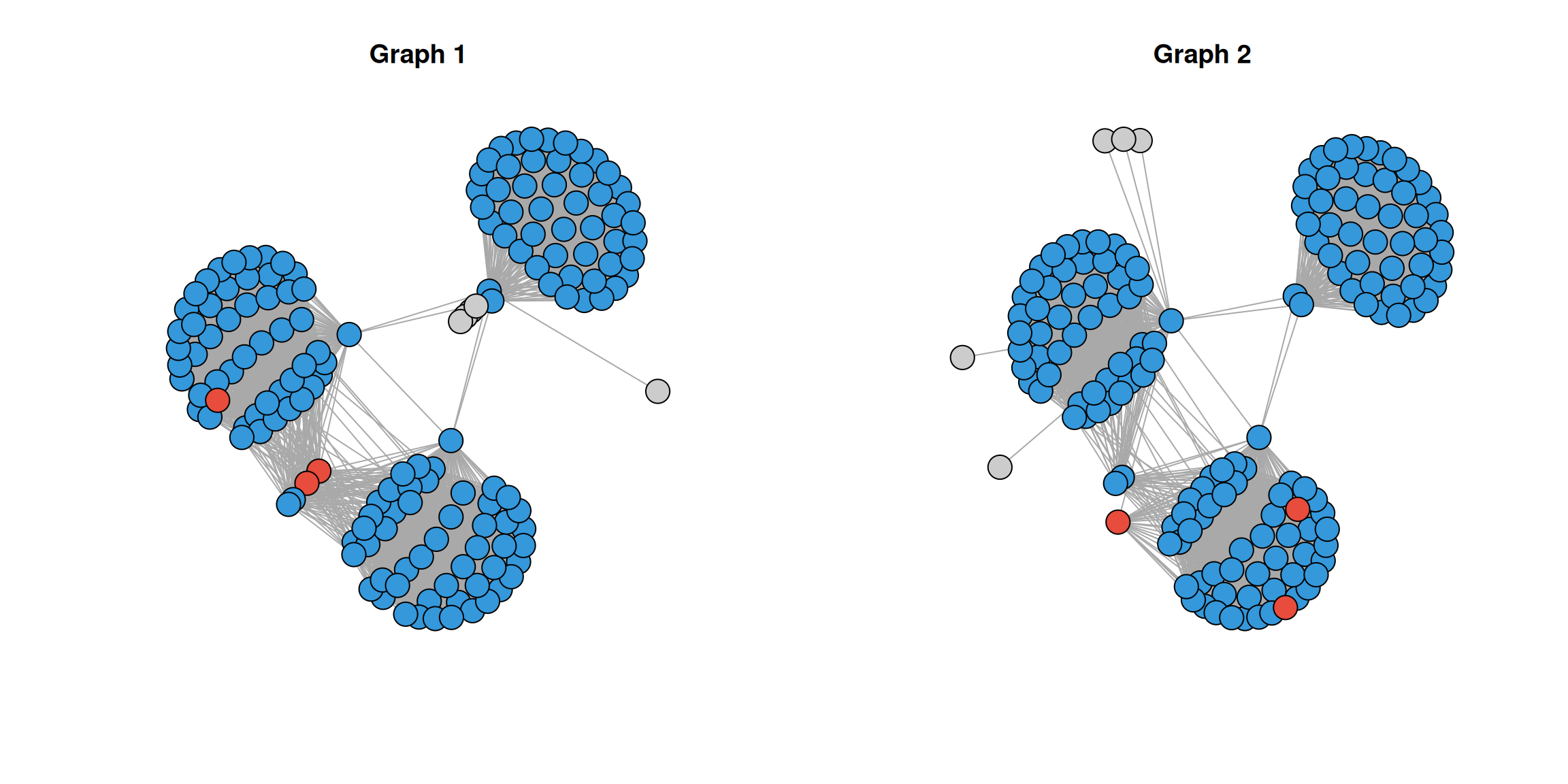
Nodes in red are those expected to show context drift. You can see the hub node loses most of its connections in graph 2, and the bridge nodes shift from spanning communities 2 and 3 to being embedded entirely within community 3.
Running EmbedDrift
Initialising the object
EmbedDrift takes the two edge tables and holds all intermediate results.
obj <- EmbedDrift(
  graph_dt_1 = test_data$g1_edges,
  graph_dt_2 = test_data$g2_edges
)

print(obj)
#> EmbedDrift
#>   Graph 1: 3917 edges | 160 nodes
#>   Graph 2: 3891 edges | 160 nodes
#>   Shared nodes: 155
#>   Graph 1 exclusive: 5
#>   Graph 2 exclusive: 5
#>   Embeddings generated: no
#>   Procrustes alignment done: no
#>   Statistics calculated: no
Generating embeddings
We train node2vec independently on both graphs using identical hyperparameters. Graph 1 serves as the reference for subsequent alignment. Given the small size of this synthetic graph, a low embedding dimension of 8 is appropriate — using a larger dimension would over-parameterise relative to the number of nodes and compress the signal we are trying to detect.
obj <- generate_initial_embeddings(
  object = obj,
  embd_dim = 8L,
  node2vec_params = params_node2vec(window_size = 2L),
  .verbose = TRUE
)
#> Embedding graph 1...
#> Embedding graph 2...

print(obj)
#> EmbedDrift
#>   Graph 1: 3917 edges | 160 nodes
#>   Graph 2: 3891 edges | 160 nodes
#>   Shared nodes: 155
#>   Graph 1 exclusive: 5
#>   Graph 2 exclusive: 5
#>   Embeddings generated: yes
#>   Procrustes alignment done: no
#>   Statistics calculated: no
If you want to get the embeddings out, getters are provided:
embd_ls <- get_embeddings(obj) # returns both matrices as a list.

embd_ls$embd_1[1:5, 1:5]
#>                dim_1      dim_2       dim_3        dim_4     dim_5
#> bridge_001 0.4196871 -0.6444453 -0.09456912  0.210284755 0.4375659
#> bridge_002 0.4418878 -0.6397567 -0.11776508  0.260207951 0.3894148
#> comm2_000  0.5842883 -0.2955315 -0.02814059  0.234892577 0.2140679
#> comm2_001  0.5220007 -0.3709379 -0.34359318 -0.077695876 0.5695884
#> comm2_002  0.5521829 -0.4003372 -0.33498651  0.007129333 0.5176302
Calculating drift
calculate_drift() aligns the two embedding matrices via Procrustes and computes per-node cosine similarities.
obj <- calculate_drift(object = obj)

stats <- get_stats(obj)
stats
#>             node cosine_similarity node_status
#>           <char>             <num>      <char>
#>   1:  bridge_001         0.7529704      shared
#>   2:  bridge_002         0.6864671      shared
#>   3:   comm2_000         0.9252533      shared
#>   4:   comm2_001         0.9866119      shared
#>   5:   comm2_002         0.9944171      shared
#>  ---
#> 161: g2_only_000         1.1000000     g2_only
#> 162: g2_only_001         1.1000000     g2_only
#> 163: g2_only_002         1.1000000     g2_only
#> 164: g2_only_003         1.1000000     g2_only
#> 165: g2_only_004         1.1000000     g2_only
The results are ordered by cosine similarity ascending, so the nodes with the greatest context drift appear first. Let’s add the ground truth labels and see whether the known differential nodes rank lower than the stable ones.
results <- merge(
  stats,
  test_data$data_info[, .(node, is_differential)],
  by = "node"
)

results[node_status == "shared"] |>
  ggplot(aes(
    x = is_differential,
    y = cosine_similarity,
    fill = is_differential
  )) +
  geom_boxplot(width = 0.4, show.legend = FALSE, outlier.shape = NA) +
  geom_jitter(width = 0.1, shape = 21, size = 3, alpha = 0.6) +
  scale_fill_manual(values = c("FALSE" = "#3498DB", "TRUE" = "#E74C3C")) +
  scale_x_discrete(labels = c("FALSE" = "Stable", "TRUE" = "Differential")) +
  labs(
    fill = "Pos Ctr"
  ) +
  theme_minimal() +
  xlab("Pos Ctr") +
  ylab("Cosine sim") +
  ggtitle("Context drift by ground truth label")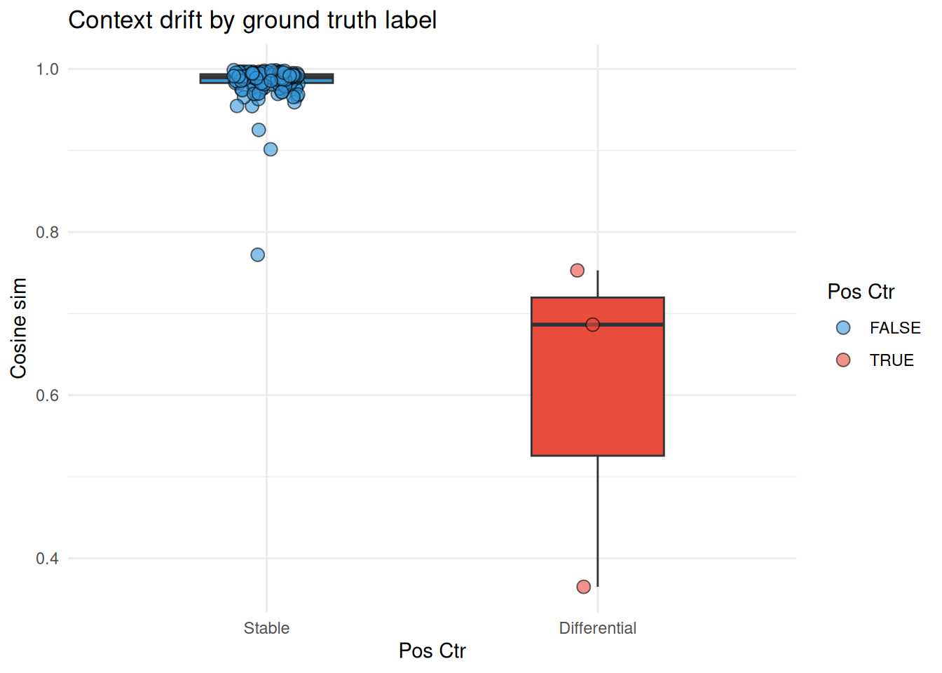
Nodes with known topological changes (hub and bridge nodes) consistently show lower cosine similarity than the stable community 1 nodes, confirming the method recovers the planted signal. The exclusive nodes carry sentinel values and are excluded from this comparison:
# exclusive nodes carry fixed sentinel values
results[node_status != "shared", .(node, cosine_similarity, node_status)]
#> Key: <node>
#>            node cosine_similarity node_status
#>          <char>             <num>      <char>
#>  1: g1_only_000              -1.1     g1_only
#>  2: g1_only_001              -1.1     g1_only
#>  3: g1_only_002              -1.1     g1_only
#>  4: g1_only_003              -1.1     g1_only
#>  5: g1_only_004              -1.1     g1_only
#>  6: g2_only_000               1.1     g2_only
#>  7: g2_only_001               1.1     g2_only
#>  8: g2_only_002               1.1     g2_only
#>  9: g2_only_003               1.1     g2_only
#> 10: g2_only_004               1.1     g2_only