Node2vec
Running node2vec
Setup
Background
Node2vec generates vector representations of nodes in a graph by running biased random walks that sample the local neighbourhood of each node, then training a skip-gram model over the resulting sequences. Nodes that appear in similar contexts across the graph will have similar embedding vectors. For a full description of the algorithm, see Grover & Leskovec.
Synthetic data
genewalkR provides quite a few synthetic graph data sets for testing and exploration purposes, namely:
- Barbell graph: a graph of two distinct clusters
- Cavemen graph: a graph with distinct communities with a low probability of connection between them.
- Stochastic blocks: a more densely connected graph with communities; however, more cross-edges compared to the previous graphs.
Exploring node2vec
Let’s check what node2vec does with different types of graphs and if the embeddings faithfully recover the graph structure.
Barbell graph
Let’s load in the barbell graph.
# this creates a random data set with 20 nodes per barbell cluster
barbell_data <- node2vec_test_data(
  test_type = "barbell",
  n_nodes_per_cluster = 20L
)
Exploring the data
Let’s transform this into an igraph first and just look at the graph as is.
g <- igraph::graph_from_data_frame(d = barbell_data$edges, directed = FALSE)

plot(g, vertex.label = NA)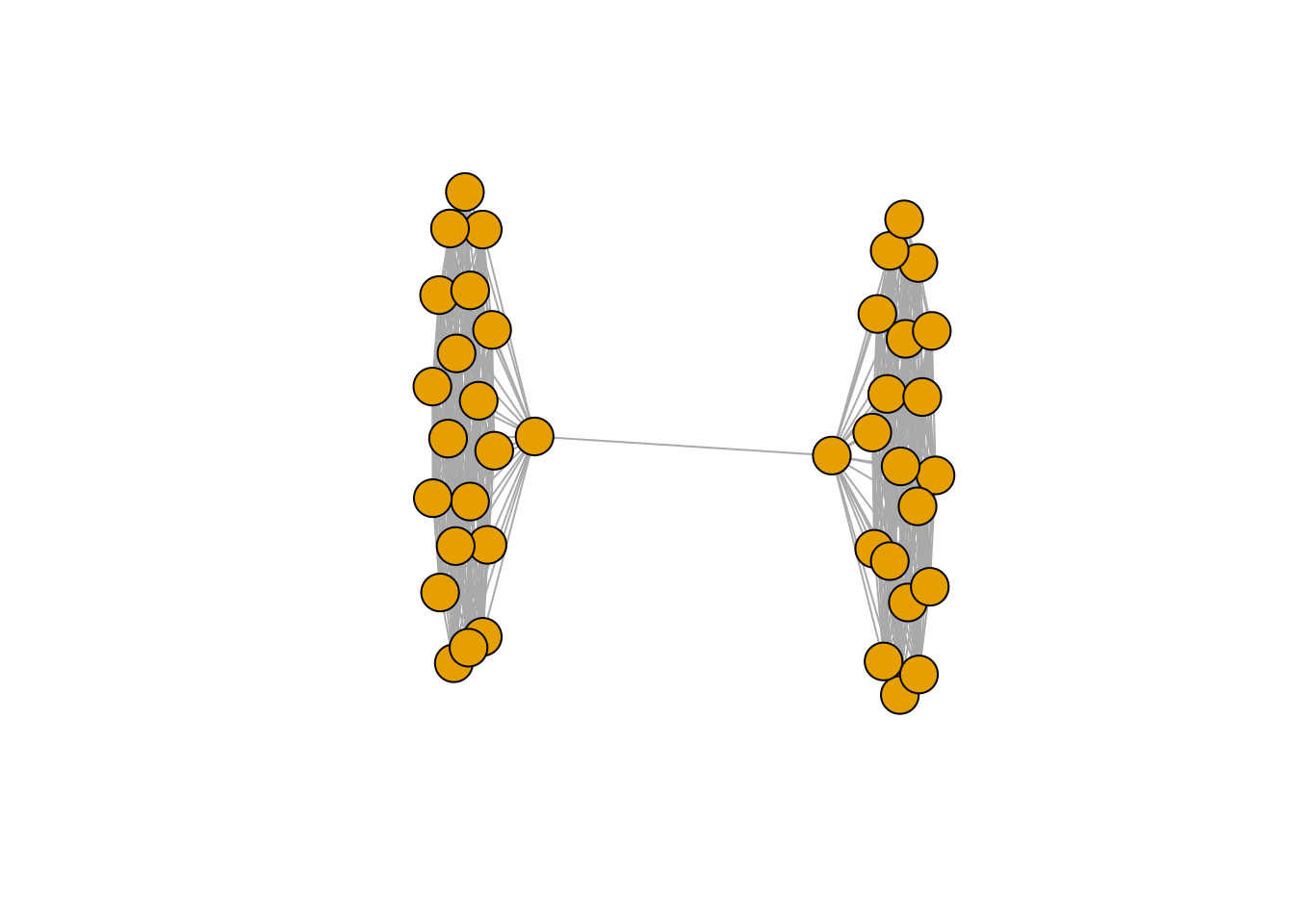
Running node2vec
You can appreciate a nice barbell graph with two distinct groups. Now let’s run node2vec on this data. The node2vec implementation is based on node2vec-rs, a Rust-based implementation of node2vec. In its default setting, we use a HIGHLY optimised version that runs on the CPU with SIMD-acceleration and a RWlock free version of SGD - known as Hogwild!. This approach is also used in the original version of word2vec, see Mikolov, et al. The issue with this is that the underlying embeddings will not be deterministic; however, the structure of the underlying graph will be identified. If you really, really, really need deterministic results here, set the parameter n_workers = 1L.
# run node2vec
barbell_node2vec_results <- node2vec(
  graph_dt = barbell_data$edges,
  .verbose = TRUE
)

# the parameters are controlled via a supplied parameter list, see code here
str(params_node2vec())
#> List of 10
#>  $ p             : num 1
#>  $ q             : num 1
#>  $ walks_per_node: int 40
#>  $ walk_length   : int 40
#>  $ num_workers   : int 2
#>  $ batch_size    : int 256
#>  $ n_epochs      : int 20
#>  $ n_negatives   : int 5
#>  $ window_size   : int 2
#>  $ lr            : num 0.01

# this list can be supplied and tells node2vec how to run
Let’s generate a PCA of the embedding and explore the first two principal components visually
# run pca on the embeddings
pca_results <- prcomp(barbell_node2vec_results, scale. = TRUE)

pca_dt <- as.data.table(pca_results$x[, 1:2], keep.rownames = "node") %>%
  merge(., barbell_data$node_labels, by = "node")

pca_dt[, cluster := factor(cluster)]

ggplot(data = pca_dt, mapping = aes(x = PC1, y = PC2)) +
  geom_point(
    mapping = aes(color = cluster),
    size = 3
  ) +
  theme_bw() +
  labs(color = "Cluster:")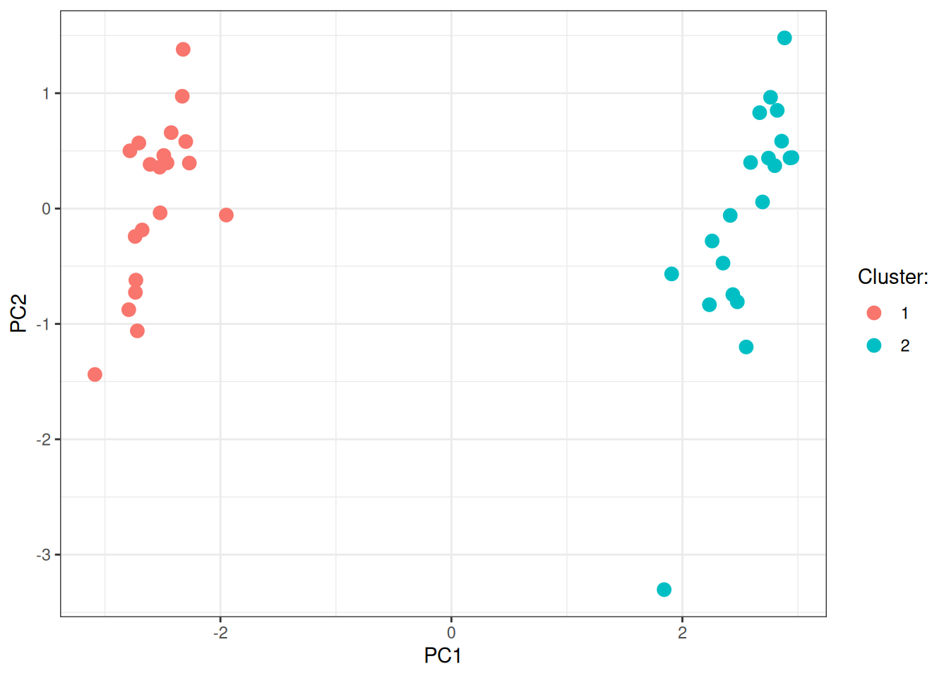
As you can appreciate, node2vec embeddings nicely identify the two groups in the underlying graph.
Cavemen graph
Visualisation of the graph structure in igraph first (same as for the previous graph):
# generate the cavemen
caveman_data <- node2vec_test_data(
  test_type = "cavemen", n_clusters = 5L, p_between = 0.5
)

g <- igraph::graph_from_data_frame(d = caveman_data$edges, directed = FALSE)

plot(g, vertex.label = NA)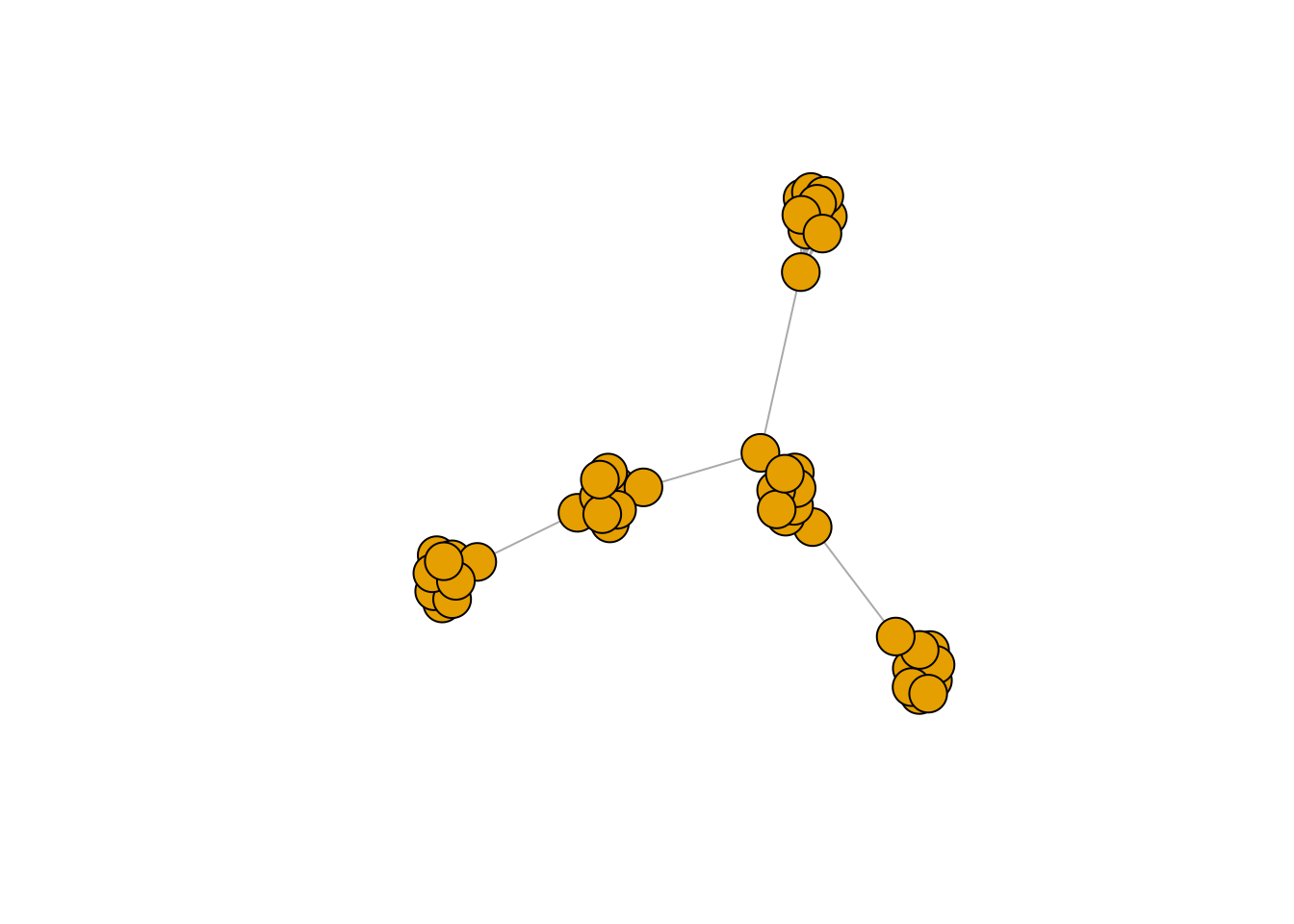
Let’s visualise the PCA on top of the embeddings generated by node2vec on this graph structure.
# run node2vec
cavemen_node2vec_results <- node2vec(
  graph_dt = caveman_data$edges,
  .verbose = TRUE
)

# run pca on the embeddings
pca_results <- prcomp(cavemen_node2vec_results, scale. = TRUE)

pca_dt <- as.data.table(pca_results$x[, 1:2], keep.rownames = "node") %>%
  merge(., caveman_data$node_labels, by = "node")

pca_dt[, cluster := factor(cluster)]

ggplot(data = pca_dt, mapping = aes(x = PC1, y = PC2)) +
  geom_point(
    mapping = aes(color = cluster),
    size = 3
  ) +
  theme_bw() +
  labs(color = "Cluster:")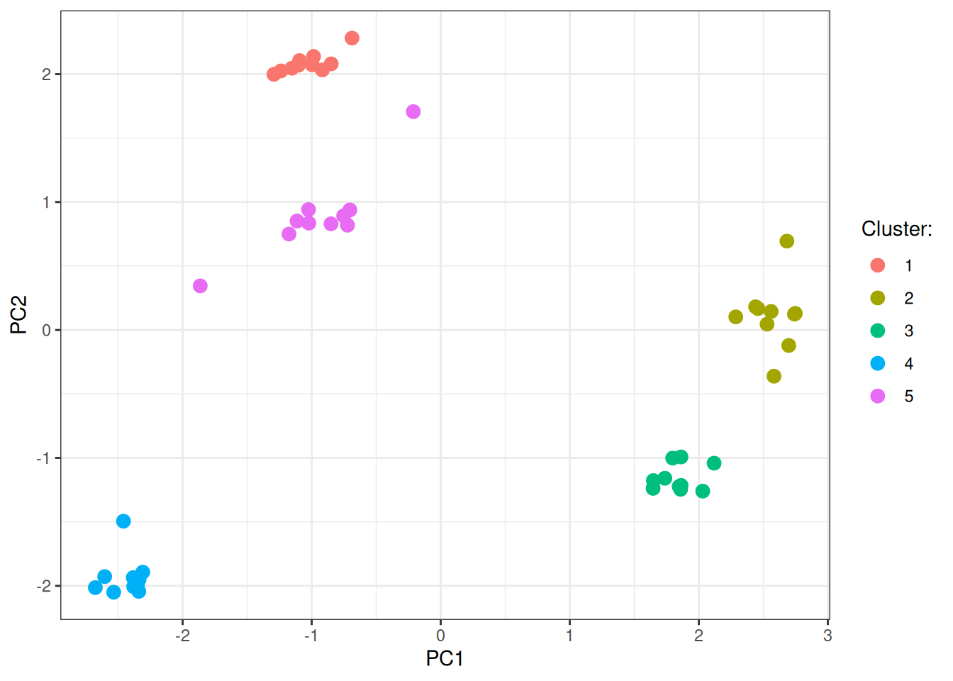
Stochastic blocks
In this last graph example, we have less defined communities with more between edges across the communities. We will do exactly what we did before.
# generate the stochastic block graph
stochastic_block_data <- node2vec_test_data(
  test_type = "stochastic_block", n_clusters = 3L, p_between = 0.05
)

g <- igraph::graph_from_data_frame(
  d = stochastic_block_data$edges,
  directed = FALSE
)

plot(g, vertex.label = NA)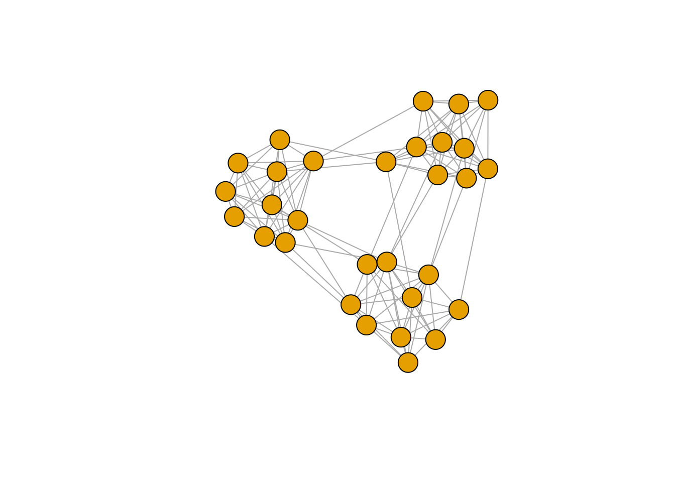
Let’s visualise again the PCA here:
# run node2vec
stochastic_blocks_node2vec_results <- node2vec(
  graph_dt = stochastic_block_data$edges,
  .verbose = TRUE
)

# run pca on the embeddings
pca_results <- prcomp(stochastic_blocks_node2vec_results, scale. = TRUE)

pca_dt <- as.data.table(pca_results$x[, 1:2], keep.rownames = "node") %>%
  merge(., stochastic_block_data$node_labels, by = "node")

pca_dt[, cluster := factor(cluster)]

ggplot(data = pca_dt, mapping = aes(x = PC1, y = PC2)) +
  geom_point(
    mapping = aes(color = cluster),
    size = 3
  ) +
  theme_bw() +
  labs(color = "Cluster:")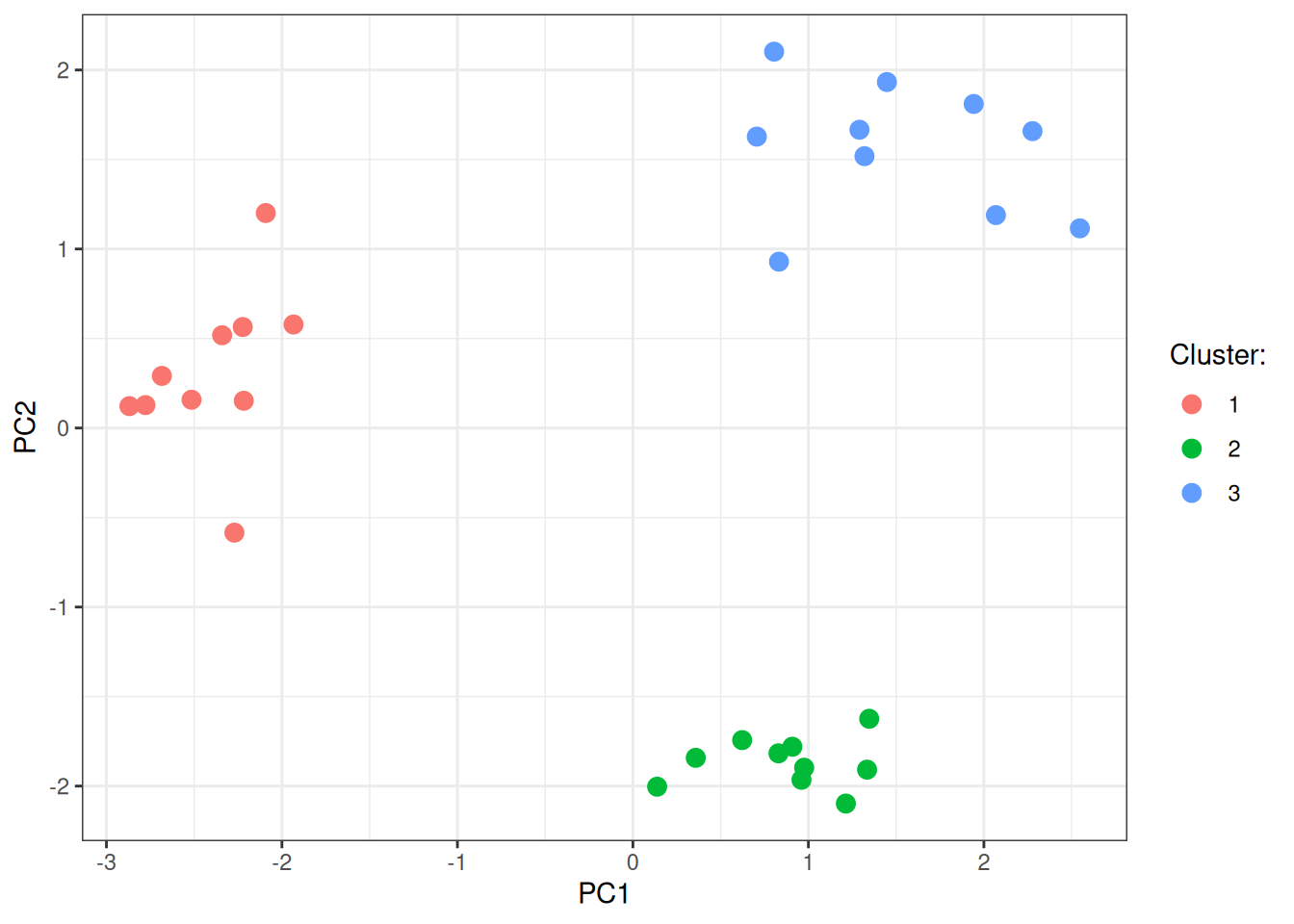
In conclusion, node2vec generates an embedding of the underlying network structure that you can then use to visualise the data or do additional analyses (with some already part of this package and more to be added). Pending on your needs, you can go high on the available workers and make this fast, or if you really, really, really need similar embeddings every single time, you can also choose to disable the parallelism during training (the random walks will still be generated via Rayon in parallel).