Running GeneWalk
Exploring Gene Walk
This vignette will first show how Gene Walk behaves on synthetic data, what assumptions are baked in and then we will move onto using it with real data. If you want to understand the method in more detail, please check out Ietswaart et al.
Setup
Synthetic data
Exploring the data and initialising the object
Let’s start with some synthetic data to understand how this works… The synthetic GeneWalk network is designed testing and benchmarking, with signal genes forming coherent, degree-matched graph neighbourhoods and noise genes spanning multiple ontology subtrees at random. The signal (“anchor”) genes will have some VERY clear signal. Noise genes also still due to the nature of the synthetic data; however, to a lesser extent.
gene_walk_syn_data <- synthetic_genewalk_data()

str(gene_walk_syn_data)
#> List of 4
#>  $ full_data       :Classes 'data.table' and 'data.frame':   8237 obs. of  3 variables:
#>   ..$ from: chr [1:8237] "term_0001" "term_0001" "term_0002" "term_0002" ...
#>   ..$ to  : chr [1:8237] "term_0002" "term_0003" "term_0004" "term_0005" ...
#>   ..$ type: chr [1:8237] "hierarchy" "hierarchy" "hierarchy" "hierarchy" ...
#>   ..- attr(*, ".internal.selfref")=<externalptr>
#>  $ gene_to_pathways:Classes 'data.table' and 'data.frame':   6399 obs. of  3 variables:
#>   ..$ from: chr [1:6399] "gene_signal_0001" "gene_signal_0001" "gene_signal_0001" "gene_signal_0001" ...
#>   ..$ to  : chr [1:6399] "term_0025" "term_0019" "term_0024" "term_0017" ...
#>   ..$ type: chr [1:6399] "part_of" "part_of" "part_of" "part_of" ...
#>   ..- attr(*, ".internal.selfref")=<externalptr>
#>  $ gene_ids        : chr [1:444] "gene_signal_0001" "gene_signal_0002" "gene_signal_0003" "gene_signal_0004" ...
#>  $ pathway_ids     : chr [1:355] "term_0001" "term_0002" "term_0003" "term_0004" ...
The data contains everything we need to initialise a new GeneWalk:
- The full_data with the term ontology, gene to gene edges and gene to terms, mimicking relevant inputs.
- The genes to pathways for testing later.
- The gene identifiers including in the run. In this case, we have a set of “signal” genes that serve as a positive control and “noise genes” that are randomly distributed.
- The term/pathway identifiers.
Let’s initialise the class.
# this create the class
genewalk_obj <- GeneWalk(
  graph_dt = gene_walk_syn_data$full_data,
  gene_to_pathway_dt = gene_walk_syn_data$gene_to_pathways,
  gene_ids = gene_walk_syn_data$gene_ids,
  pathway_ids = gene_walk_syn_data$pathway_ids
)

genewalk_obj
#> GeneWalk
#>   Represented genes gene_signal_0001 | gene_signal_0002 | gene_signal_0003 ; Total of 444 genes.
#>   Number of edges: 8237
#>   Edge distribution:
#>     Hierarchy (654)
#>     Part of (6399)
#>     Interaction (1184)
#>   Embedding generated: no
#>   Permutations generated: no
#>   Statistics calculated: no
Running gene walk on the synthetic data
This function here generates the node2vec embedding based on the network. To avoid instability issues due to the Hogwild!-type SGD used, we limit the threads to 1L here via params_genewalk(). If you want to do fast testing (for parameter optimisation), you can increase this to more. Initially, we generate n_graph initial representations. The authors of the original work default to 3L here. A potential approach could be to leverage the more cores and run more iterations. The SGD scales basically linearly with the number of threads you use.
genewalk_obj <- generate_initial_emb(
  genewalk_obj,
  n_graph = 3L,
  genewalk_params = params_genewalk(),
  .verbose = TRUE
)
We need to generate a background distribution for testing purposes. This will generate three random permuted networks as in the paper. These will be used for statistical testing.
genewalk_obj <- generate_permuted_emb(genewalk_obj, .verbose = TRUE)We now need to compare the similarity of the Cosine similarities between the gene embeddings to the pathway embeddings and check how often they are larger than the ones from the background embedding, giving us the p-values.
genewalk_obj <- calculate_genewalk_stats(
  genewalk_obj,
  .verbose = TRUE
)
Now we can extract the statistics:
statistics <- get_stats(genewalk_obj)

head(statistics)
#>                  gene   pathway similarity    sem_sim     avg_pval
#>                <char>    <char>      <num>      <num>        <num>
#> 1: gene_anchor_1_0015 term_0070  0.9551714 0.01860447 0.0002820349
#> 2: gene_anchor_1_0003 term_0070  0.9539643 0.01328374 0.0004367785
#> 3: gene_anchor_4_0010 term_0156  0.9343623 0.01708196 0.0011255221
#> 4: gene_anchor_4_0005 term_0156  0.9317070 0.00685643 0.0015102091
#> 5: gene_anchor_4_0002 term_0156  0.9297756 0.01473127 0.0016251556
#> 6: gene_anchor_1_0004 term_0082  0.9269314 0.01442637 0.0017465073
#>    pval_ci_lower pval_ci_upper avg_global_fdr global_fdr_ci_lower
#>            <num>         <num>          <num>               <num>
#> 1:  0.0000265351   0.002997678      0.1996261           0.1762366
#> 2:  0.0001206405   0.001581355      0.1996261           0.1762366
#> 3:  0.0002112360   0.005997083      0.1996261           0.1762366
#> 4:  0.0008796587   0.002592746      0.1996261           0.1762366
#> 5:  0.0005268030   0.005013507      0.1996261           0.1762366
#> 6:  0.0005465031   0.005581465      0.1996261           0.1762366
#>    global_fdr_ci_upper avg_gene_fdr gene_fdr_ci_lower gene_fdr_ci_upper
#>                  <num>        <num>             <num>             <num>
#> 1:           0.2261198  0.005151888      0.0005704578        0.04652746
#> 2:           0.2261198  0.006551678      0.0018096074        0.02372033
#> 3:           0.2261198  0.012380743      0.0023235965        0.06596791
#> 4:           0.2261198  0.022653137      0.0131948805        0.03889119
#> 5:           0.2261198  0.021114187      0.0068523342        0.06505942
#> 6:           0.2261198  0.009536346      0.0072132993        0.01260753
The different metrics in the data Let’s explore the signal in the synthetic data a bit… What are we observing … ?
# add the labels for signal and noise
statistics[, signal := grepl("anchor", gene)][,
  signal := factor(signal, levels = c("TRUE", "FALSE"))
]

# plot the gene <> term similarities
ggplot(
  data = statistics,
  mapping = aes(x = similarity)
) +
  geom_histogram(bins = 45, fill = "lightgrey") +
  facet_wrap(~ signal) +
  xlab("Cosine similarity") +
  ylab("Count") +
  theme_bw()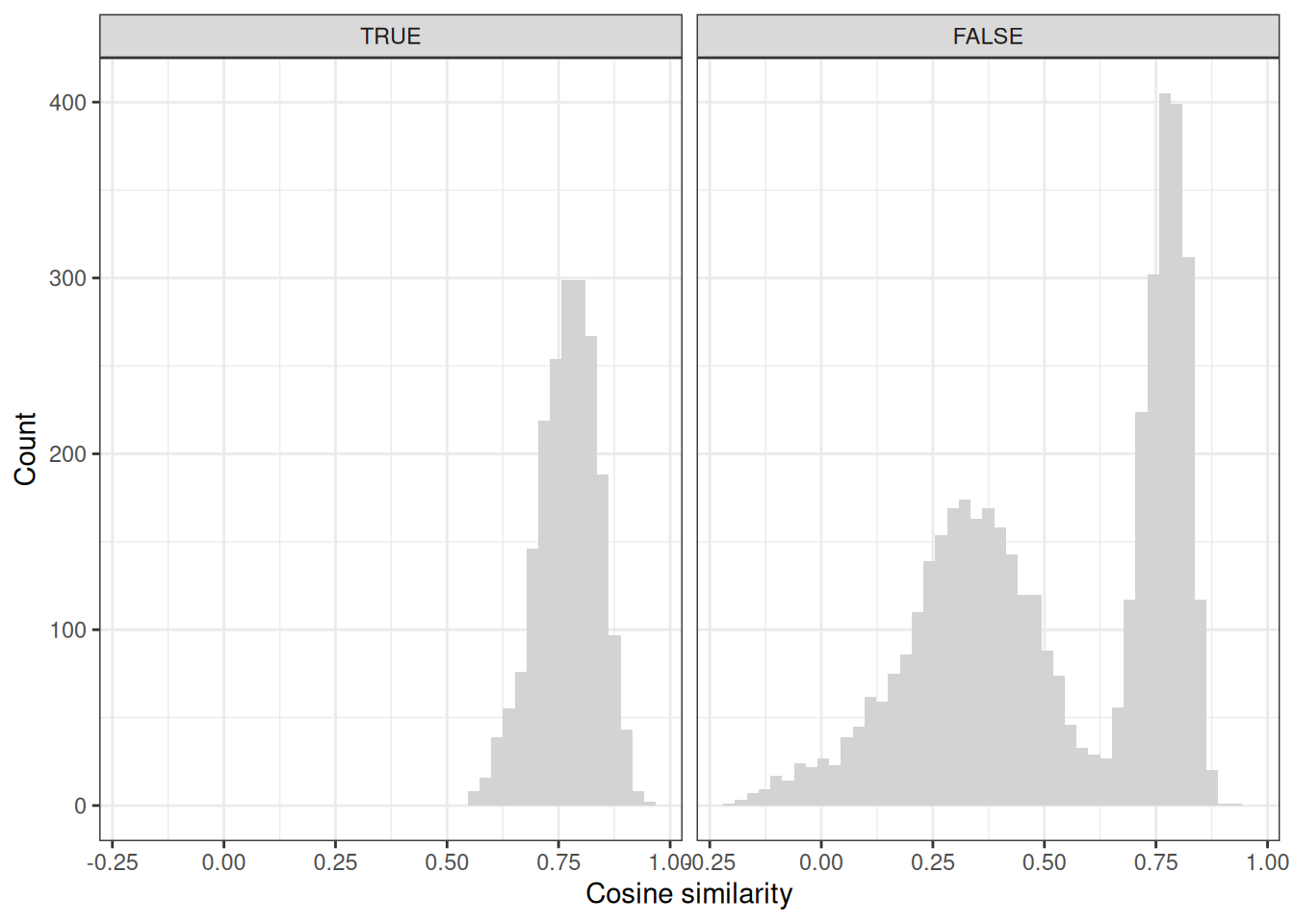
As we can appreciate, the Cosine similarities between the genes and pathways in the signal data set are all much higher compared to the FALSE ones, and we have a bimodal distribution for the noise genes. Some of these just by accident get connected into the same dense communities from the signal genes, but a large number of them are just noise. Let’s check the p-values
ggplot(
  data = statistics,
  mapping = aes(x = avg_pval)
) +
  geom_histogram(bins = 45, fill = "lightgrey") +
  facet_wrap(~ signal) +
  xlab("p-val") +
  ylab("Count") +
  theme_bw()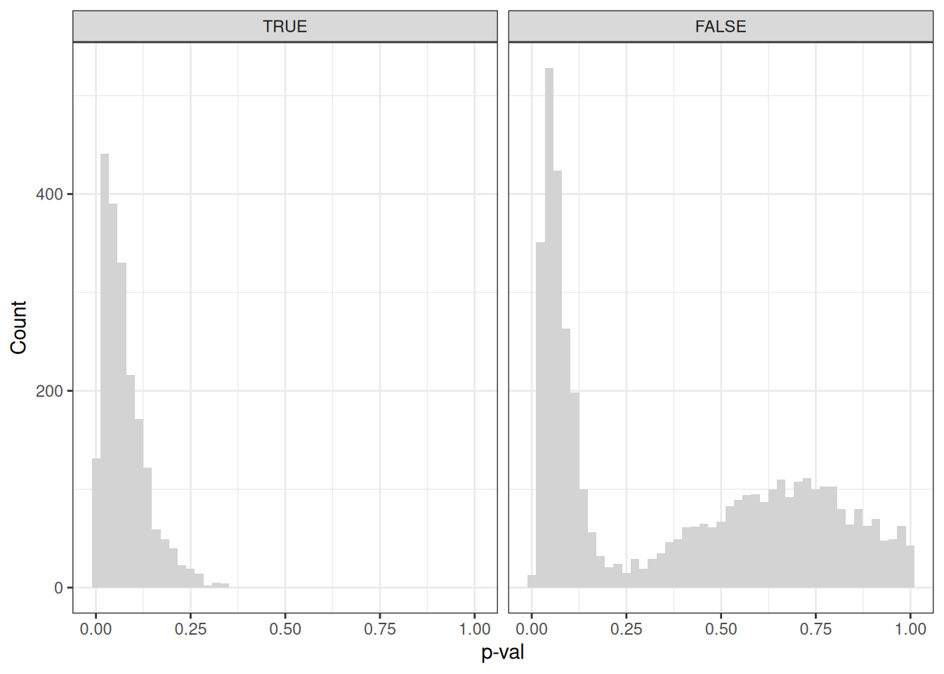
The patterns of the Cosine similarities are reproduced here.
We can appreciate that 50% of the signal genes have a significantly higher cosine similarity in the embedding space with their connected pathway. For the random genes, it’s only ~20%. But now let’s move on to some real data.
Real data
Let’s explore real data now. The package provides a builder factory to generate the objects. Within the package, there is a DuckDB that contains:
Network resources
- The STRING network extracted from OpenTargets.
- The SIGNOR network extracted from OpenTargets.
- The Reactome gene to gene network extracted from OpenTargets.
- The Intact network extracted from OpenTargets.
- The Pathway Commons interactions, see Rodchenkov, et al..
- A combined network from the sources above, based on the approach from Barrio-Hernandez, et al..
Pathway terms
- The Gene Ontology data extracted from the OBO files from the OBO foundry and OpenTargets.
- The Reactome pathway ontology and their gene to pathway associations from OpenTargets.
Using the builder factory
Let’s use the Gene Ontology and combined network for this example. If you do this for the first time, the database will be downloaded into your cache. If you wish to reset the DB and re-download it (for example for a new release), you can use reload_db().
gw_factory <- GeneWalkGenerator$new()

gw_factory$add_pathways() # will add GO to the builder
gw_factory$add_ppi(source = "combined") # will add the combined one
gw_factory$build() # will load the data into the factory
#> Downloading database...
#> Download complete
#> Built network with 2646428 edges and 61982 nodes
The idea of the factory is to easily iterate through various bags of genes of interest. Now let’s use the factory to look specifically at the MYC target genes (provided in the package and extracted from the Hallmarks MYC V1 gene set, see Liberzon et al.) and generate a GeneWalkNetwork for them.
data(myc_genes)

myc_gwn <- gw_factory$create_for_genes(genes = myc_genes$ensembl_gene)

myc_gwn
#> GeneWalk
#>   Represented genes ENSG00000004779 | ENSG00000013275 | ENSG00000041357 ; Total of 200 genes.
#>   Number of edges: 86990
#>   Edge distribution:
#>     Interaction (6149)
#>     Part of (5598)
#>     Hierarchy (75243)
#>   Embedding generated: no
#>   Permutations generated: no
#>   Statistics calculated: no
Check the node degree
For GeneWalk to optimally work, you need quite a few edges based on the interaction networks. This is a helper to get some information on the underlying node degree:
check_degree_distribution(myc_gwn)
#>
#> --- hierarchy ---
#>    Min. 1st Qu.  Median    Mean 3rd Qu.    Max.
#>   1.000   1.000   3.000   3.885   4.000 435.000
#>
#> --- interaction ---
#>    Min. 1st Qu.  Median    Mean 3rd Qu.    Max.
#>     1.0    32.0    58.0    61.8    82.0   238.0
#>
#> --- part_of ---
#>    Min. 1st Qu.  Median    Mean 3rd Qu.    Max.
#>    1.00    1.00    1.00    5.73    4.00  191.00
We can appreciate quite a few interactions between the genes and also decent number of connections in the PPPI network. We can proceed here. Should you observe a low number of interaction connections, likely, your gene set is too small (or noisy) and the approach will not work well (or rather as expected with lack of signal).
Running gene walk on actual data
We can now use the same steps as above. Generate first three iterations of the real embedding based on different random seeds:
# we are reducing the number of walks here... the original paper used 100L
# walks per node with walk_length = 10L. you can play around with the parameters
# here.

# this will take a bit
myc_gwn <- generate_initial_emb(
  myc_gwn,
  genewalk_params = params_genewalk(walks_per_node = 25L),
  .verbose = TRUE
)

# this, too
myc_gwn <- generate_permuted_emb(
  myc_gwn,
  .verbose = TRUE
)

# let's calculate the statistics
myc_gwn <- calculate_genewalk_stats(
  myc_gwn,
  .verbose = TRUE
)

# let's extract the results
myc_gwn_res <- get_stats(myc_gwn)
Exploring the results
Check the embeddings
Let’s compare the embeddings we generate against the NULLs
plot_similarities(myc_gwn)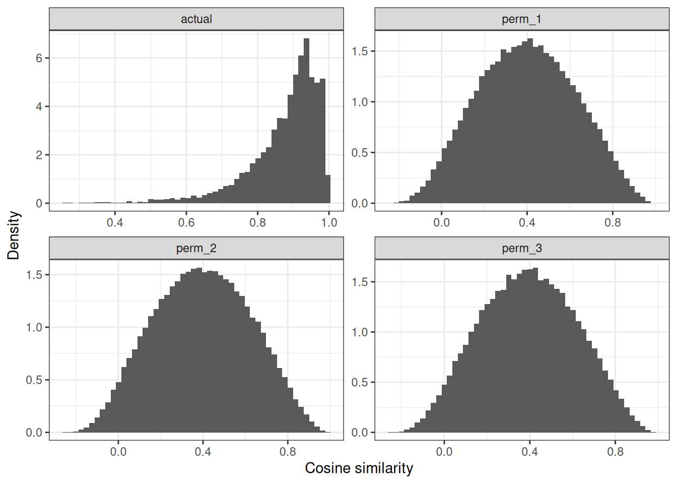
We can appreciate that we have clearly some genes with higher similarities to their connected GO terms compared to the three NULLs. This is expected, as these genes are highly studied and connected.
Scatter plot
A simple way to visualise the initial results is to use the plot_results() function. This will tell you the connectivity of the genes within your bag of genes (degree + 1 on the x-axis), the number of gene <> pathway connections that are significant for this specific gene and the number of gene <> pathway connections.
plot_gw_results(myc_gwn, fdr_treshold = 0.05)Other options are to plot for individual genes the significantly associated terms (not shown).
Actual data
# translate go ids to names and do the same for the gene symbols
gene_symbol_translation <- setNames(
  myc_genes$gene_symbol,
  myc_genes$ensembl_gene
)

# get the go data
go_info <- get_gene_ontology_info()

go_id_translation <- setNames(
  go_info$go_name,
  go_info$go_id
)

myc_gwn_res_translated <- copy(myc_gwn_res)[, `:=`(
  gene = gene_symbol_translation[gene],
  pathway = go_id_translation[pathway]
)]

head(myc_gwn_res_translated, 10L)
#>       gene                               pathway similarity      sem_sim
#>     <char>                                <char>      <num>        <num>
#>  1: SNRPB2       U2-type prespliceosome assembly  0.9968249 0.0008473674
#>  2:  RPL34                    cytosolic ribosome  0.9961501 0.0025251946
#>  3:   MCM7 single-stranded DNA helicase activity  0.9952804 0.0023510163
#>  4: SNRPB2              precatalytic spliceosome  0.9949466 0.0025986310
#>  5:   RRP9                        snoRNA binding  0.9948157 0.0004635765
#>  6:  RPL34     cytosolic large ribosomal subunit  0.9942588 0.0032039076
#>  7:   MCM4 single-stranded DNA helicase activity  0.9941259 0.0020458616
#>  8: SNRPD2       U2-type prespliceosome assembly  0.9940280 0.0024073063
#>  9: EIF4A1            cytoplasmic stress granule  0.9939549 0.0020944587
#> 10:   RPL6     cytosolic large ribosomal subunit  0.9939253 0.0019984519
#>         avg_pval pval_ci_lower pval_ci_upper avg_global_fdr global_fdr_ci_lower
#>            <num>         <num>         <num>          <num>               <num>
#>  1: 1.000000e-16  1.000000e-16  1.000000e-16   4.389406e-15        2.929681e-15
#>  2: 1.000000e-16  1.000000e-16  1.000000e-16   4.389406e-15        2.929681e-15
#>  3: 1.000000e-16  1.000000e-16  1.000000e-16   4.389406e-15        2.929681e-15
#>  4: 5.397352e-13  1.016173e-19  2.866777e-06   1.330640e-11        1.395357e-18
#>  5: 1.000000e-16  1.000000e-16  1.000000e-16   4.389406e-15        2.929681e-15
#>  6: 6.800498e-13  8.140565e-20  5.681027e-06   1.607500e-11        2.204230e-18
#>  7: 5.397352e-13  1.016173e-19  2.866777e-06   1.399173e-11        2.518252e-18
#>  8: 6.800498e-13  8.140565e-20  5.681027e-06   1.463260e-11        1.273725e-18
#>  9: 5.397352e-13  1.016173e-19  2.866777e-06   1.396794e-11        2.329096e-18
#> 10: 5.397352e-13  1.016173e-19  2.866777e-06   1.399173e-11        2.518252e-18
#>     global_fdr_ci_upper avg_gene_fdr gene_fdr_ci_lower gene_fdr_ci_upper
#>                   <num>        <num>             <num>             <num>
#>  1:        6.576444e-15 4.367481e-16      1.767391e-16      1.079269e-15
#>  2:        6.576444e-15 1.138562e-15      7.485793e-16      1.731713e-15
#>  3:        6.576444e-15 1.400000e-15      1.400000e-15      1.400000e-15
#>  4:        1.268924e-04 1.310763e-12      1.215881e-19      1.413049e-05
#>  5:        6.576444e-15 8.454072e-16      4.528455e-16      1.578272e-15
#>  6:        1.172317e-04 4.136708e-12      3.372801e-19      5.073633e-05
#>  7:        7.773984e-05 6.386671e-12      1.236338e-18      3.299225e-05
#>  8:        1.680998e-04 1.737007e-12      9.001490e-20      3.351883e-05
#>  9:        8.376787e-05 5.547066e-12      3.905015e-19      7.879595e-05
#> 10:        7.773984e-05 3.956615e-12      4.408788e-19      3.550817e-05
Why is so much significant here? Is this not just pathway enrichment? Well no. GeneWalk only tests for pre-existing edges of a gene against the pathway, given the context of the pathway ontology AND the interactions between the genes. It is more a gene prioritisation/contextualisation tool than a classical pathway enrichment. Nonetheless, let’s check what happens with noisy data…
Random data set
genes <- get_gene_info() %>%
  .[biotype == "protein_coding"]

set.seed(123L)

random_gene_set <- sample(genes$ensembl_id, 200L)

random_gwn <- gw_factory$create_for_genes(genes = random_gene_set)
#> Warning in get_gw_data_filtered.DataBuilder(x = private$gene_walk_data, : 10
#> gene(s) had no edges in the network and were excluded: ENSG00000274944,
#> ENSG00000223601, ENSG00000224383, ENSG00000235034, ENSG00000286022,
#> ENSG00000180425, ENSG00000261611, ENSG00000263715, ENSG00000268870,
#> ENSG00000187808

# we can appreciate that we only have very few interactions between the genes
random_gwn
#> GeneWalk
#>   Represented genes ENSG00000004939 | ENSG00000006837 | ENSG00000007968 ; Total of 190 genes.
#>   Number of edges: 78815
#>   Edge distribution:
#>     Interaction (290)
#>     Part of (3282)
#>     Hierarchy (75243)
#>   Embedding generated: no
#>   Permutations generated: no
#>   Statistics calculated: no
Let’s run fast with as many threads as possible the rest
# we will parallelise this over all available threads, as we do not care
# about determinism in the results
no_threads <- parallel::detectCores()

random_gwn <- generate_initial_emb(
  random_gwn,
  genewalk_params = params_genewalk(
    walks_per_node = 25L,
    num_workers = no_threads),
  .verbose = TRUE
)

random_gwn <- generate_permuted_emb(
  random_gwn,
  .verbose = TRUE
)

random_gwn <- calculate_genewalk_stats(
  random_gwn,
  .verbose = TRUE
)

random_gwn_res <- get_stats(random_gwn)
Let’s plot the results
# that looks way worse than for the MYC genes...
plot_similarities(random_gwn)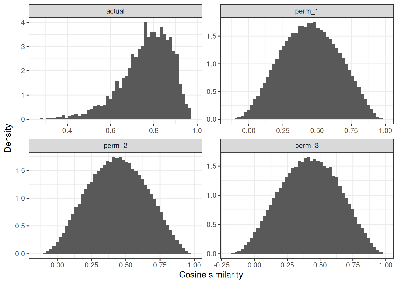
# some genes still reach significance - this is likely driven by the
# structure provided, by the gene ontology graph, but one can appreciate
# that for random genes, the thresholds fall apart
plot_gw_results(random_gwn, fdr_treshold = 0.05)
Using your own data
What if you do not want to use the provided data … ? In this case, you can use this simple wrapper class to help you. Let’s show case this in terms of the internally stored Reactome data.
# these are helpers to get the reactome data from the DuckDB in the
# package
reactome_genes <- get_gene_to_reactome()
reactome_ppi <- get_interactions_reactome()
reactome_hierarchy <- get_reactome_hierarchy(relationship = "parent_of")

data_builder <- new_data_builder(
  ppis = reactome_ppi,
  gene_to_pathways = reactome_genes,
  pathway_hierarchy = reactome_hierarchy
)
If you want to now get the full graph dt including everything for verification:
get_gw_data(data_builder) %>% head()
#>               from              to        type
#>             <char>          <char>      <char>
#> 1: ENSG00000211810 ENSG00000198851 interaction
#> 2: ENSG00000211592 ENSG00000143226 interaction
#> 3: ENSG00000211893 ENSG00000211592 interaction
#> 4: ENSG00000211790 ENSG00000231389 interaction
#> 5: ENSG00000211892 ENSG00000062598 interaction
#> 6: ENSG00000211799 ENSG00000158473 interaction
If you want to subset to your bag of genes of interest, you can run the following:
genes_of_interest <- reactome_genes[to == "R-HSA-1989781", from]

gwr_data <- get_gw_data_filtered(data_builder, genes_of_interest)

str(gwr_data)
#> List of 4
#>  $ gwn                 :Classes 'data.table' and 'data.frame':   4007 obs. of  3 variables:
#>   ..$ from: chr [1:4007] "ENSG00000120837" "ENSG00000112237" "ENSG00000196498" "ENSG00000204231" ...
#>   ..$ to  : chr [1:4007] "ENSG00000072310" "ENSG00000132964" "ENSG00000171720" "ENSG00000025434" ...
#>   ..$ type: chr [1:4007] "interaction" "interaction" "interaction" "interaction" ...
#>   ..- attr(*, ".internal.selfref")=<externalptr>
#>  $ genes_to_pathways   :Classes 'data.table' and 'data.frame':   898 obs. of  3 variables:
#>   ..$ from: chr [1:898] "ENSG00000001167" "ENSG00000001167" "ENSG00000001167" "ENSG00000001167" ...
#>   ..$ to  : chr [1:898] "R-HSA-9614657" "R-HSA-1989781" "R-HSA-380994" "R-HSA-381183" ...
#>   ..$ type: chr [1:898] "part_of" "part_of" "part_of" "part_of" ...
#>   ..- attr(*, ".internal.selfref")=<externalptr>
#>  $ represented_genes   : chr [1:116] "ENSG00000120837" "ENSG00000112237" "ENSG00000196498" "ENSG00000204231" ...
#>  $ represented_pathways: chr [1:2825] "R-HSA-9614657" "R-HSA-1989781" "R-HSA-380994" "R-HSA-381183" ...
The data can be easily supplied now:
From here on, you can run the whole approach on your custom network.