library(bixverse.gpu)
library(manifoldsR)
library(data.table)
#> Warning: package 'data.table' was built under R version 4.5.2
library(ggplot2)
#> Warning: package 'ggplot2' was built under R version 4.5.2
GPU-accelerated t-SNE
2026-09-24
Intro
bixverse.gpu provides a t-SNE wrapper via tsne_gpu() where the usually time-consuming kNN step runs on the GPU. The optimiser itself (Barnes-Hut or FFT-accelerated interpolation) is still on the CPU via the fast Rust implementation in manifoldsR.
If you want the algorithm background (perplexity, exaggeration schedules, BH vs FFT, when to reach for t-SNE over UMAP), read the manifoldsR t-SNE vignette. This vignette only covers what’s different here: the kNN runs on the GPU.
Current split of work:
-
kNN graph construction: GPU. Three backends (
"nndescent","ivf","exhaustive"). -
Affinity computation and gradient descent (BH or FFT): CPU. Same fast Rust implementation as
manifoldsR::tsne(). A GPU optimiser is on the roadmap.
For medium-sized data the kNN is usually the dominant cost, so pushing it to the GPU is the main win. On very large data the optimiser starts to dominate and the GPU advantage narrows until the optimiser also moves over.
Note
Vignettes were built locally on a MacBook Pro M1 Max. The GH runners were just too slow and do not have proper GPU support. This gives an idea of speed on a decent, but older machine.
Generating data
Same clustered synthetic data as in the UMAP vignette.
set.seed(42L)

cluster_data <- manifold_synthetic_data(
  type = "clusters",
  n_samples = 5000L,
  dim = 32L,
  parameters = params_clusters(n_clusters = 25L)
)
Running t-SNE on GPU
Default call: NN-descent on GPU for kNN, PCA init, Barnes-Hut optimiser on CPU.
tsne_default <- tsne_gpu(
  data = cluster_data$data,
  perplexity = 15,
  knn_method = "nndescent",
  tsne_params = params_tsne_gpu(),
  seed = 42L,
  .verbose = TRUE
)

plot_df <- as.data.table(tsne_default) |>
  setnames(c("tSNE1", "tSNE2"))
plot_df[, cluster := as.factor(cluster_data$membership)]

ggplot(plot_df, aes(x = tSNE1, y = tSNE2)) +
  geom_point(aes(colour = cluster), size = 0.5, alpha = 0.5) +
  theme_bw() +
  theme(legend.position = "none") +
  ggtitle("tsne_gpu, default (NN-descent + BH)")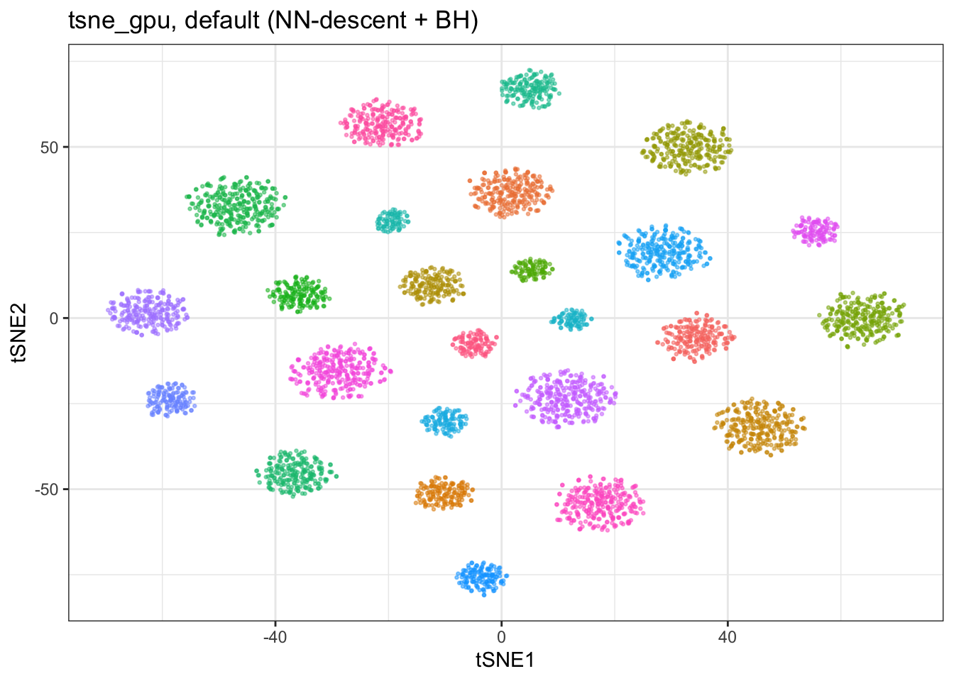
Clusters separate cleanly, as expected from t-SNE.
Choosing a kNN backend
Three GPU backends via knn_method:
-
"exhaustive": exact brute force. Small data or ground-truth checks. Quadratic in N. -
"ivf": inverted file index over Voronoi cells. Wins on large data where an approximate answer is fine. Works very well on strongly clustered data. -
"nndescent": NN-descent with CAGRA-style graph pruning. Solid default.
Tuning knobs live in params_nn_gpu(), defaults are fine for most cases. The knobs are identical to the ones described in the UMAP vignette.
IVF backend
tsne_ivf <- tsne_gpu(
  data = cluster_data$data,
  perplexity = 15,
  knn_method = "ivf",
  tsne_params = params_tsne_gpu(),
  seed = 42L,
  .verbose = TRUE
)

plot_df_ivf <- as.data.table(tsne_ivf) |>
  setnames(c("tSNE1", "tSNE2"))
plot_df_ivf[, cluster := as.factor(cluster_data$membership)]

ggplot(plot_df_ivf, aes(x = tSNE1, y = tSNE2)) +
  geom_point(aes(colour = cluster), size = 0.5, alpha = 0.5) +
  theme_bw() +
  theme(legend.position = "none") +
  ggtitle("tsne_gpu, IVF kNN")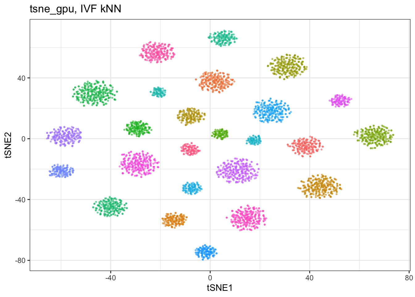
Structurally the embeddings agree. Differences are within the noise of t-SNE’s non-deterministic optimisation.
Exhaustive backend
tsne_exhaustive <- tsne_gpu(
  data = cluster_data$data,
  perplexity = 15,
  knn_method = "exhaustive",
  tsne_params = params_tsne_gpu(),
  seed = 42L,
  .verbose = TRUE
)

plot_df_exhaustive <- as.data.table(tsne_exhaustive) |>
  setnames(c("tSNE1", "tSNE2"))
plot_df_exhaustive[, cluster := as.factor(cluster_data$membership)]

ggplot(plot_df_exhaustive, aes(x = tSNE1, y = tSNE2)) +
  geom_point(aes(colour = cluster), size = 0.5, alpha = 0.5) +
  theme_bw() +
  theme(legend.position = "none") +
  ggtitle("tsne_gpu, exhaustive kNN")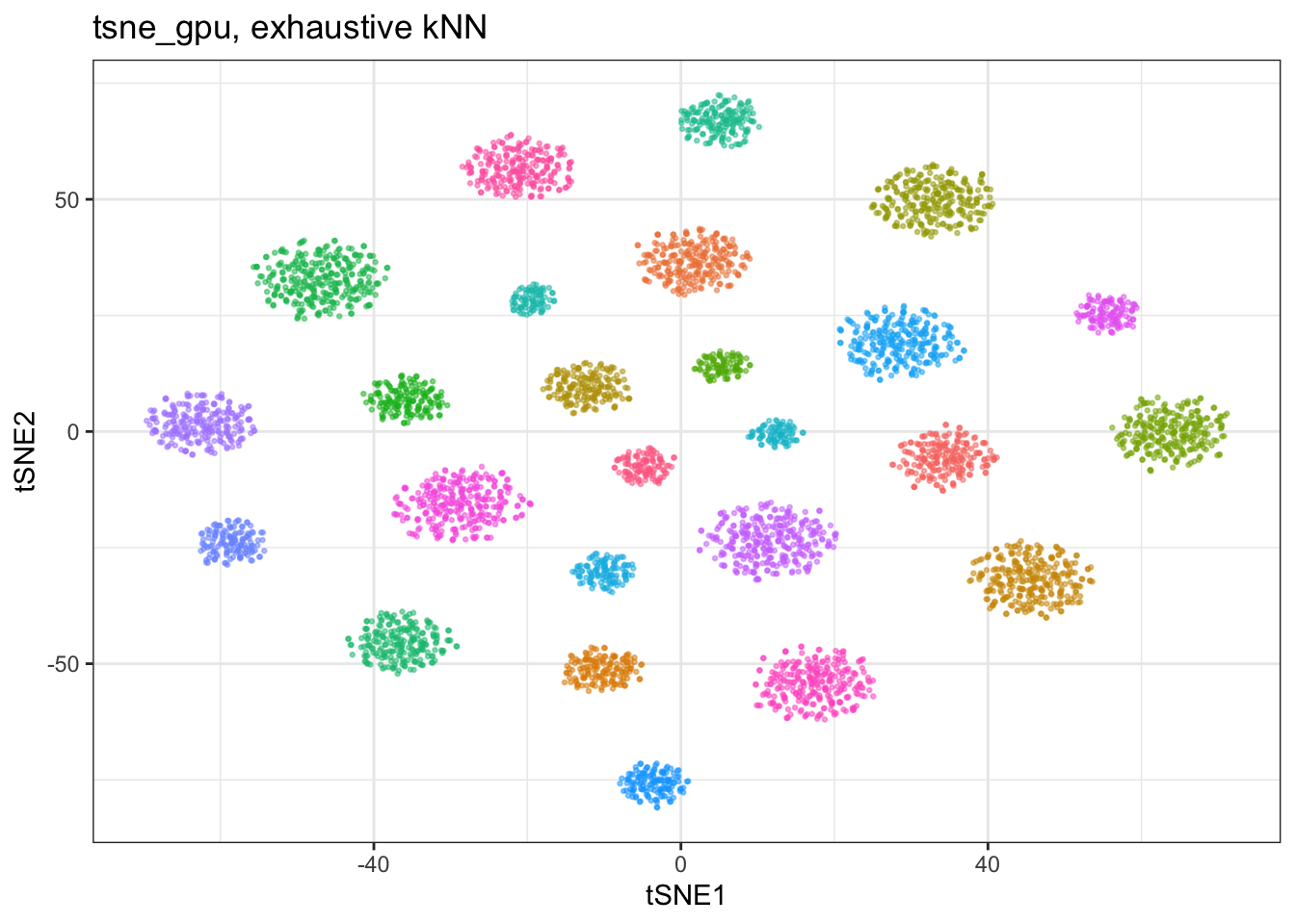
Structurally the embeddings agree. Differences are within the noise of t-SNE’s non-deterministic optimisation.
FFT-accelerated t-SNE
For large data the FFT variant reduces the optimiser cost from O(N log N) to O(N) at the price of a larger constant. Interesting at ≥ 100k samples. FFT is Unix-only (FFTW cross-compilation constraint).
tsne_fft <- tsne_gpu(
  data = cluster_data$data,
  perplexity = 15,
  approx_type = "fft",
  knn_method = "nndescent",
  tsne_params = params_tsne_gpu(),
  seed = 42L,
  .verbose = TRUE
)

plot_df_fft <- as.data.table(tsne_fft) |>
  setnames(c("tSNE1", "tSNE2"))
plot_df_fft[, cluster := as.factor(cluster_data$membership)]

ggplot(plot_df_fft, aes(x = tSNE1, y = tSNE2)) +
  geom_point(aes(colour = cluster), size = 0.5, alpha = 0.5) +
  theme_bw() +
  theme(legend.position = "none") +
  ggtitle("tsne_gpu, FFT")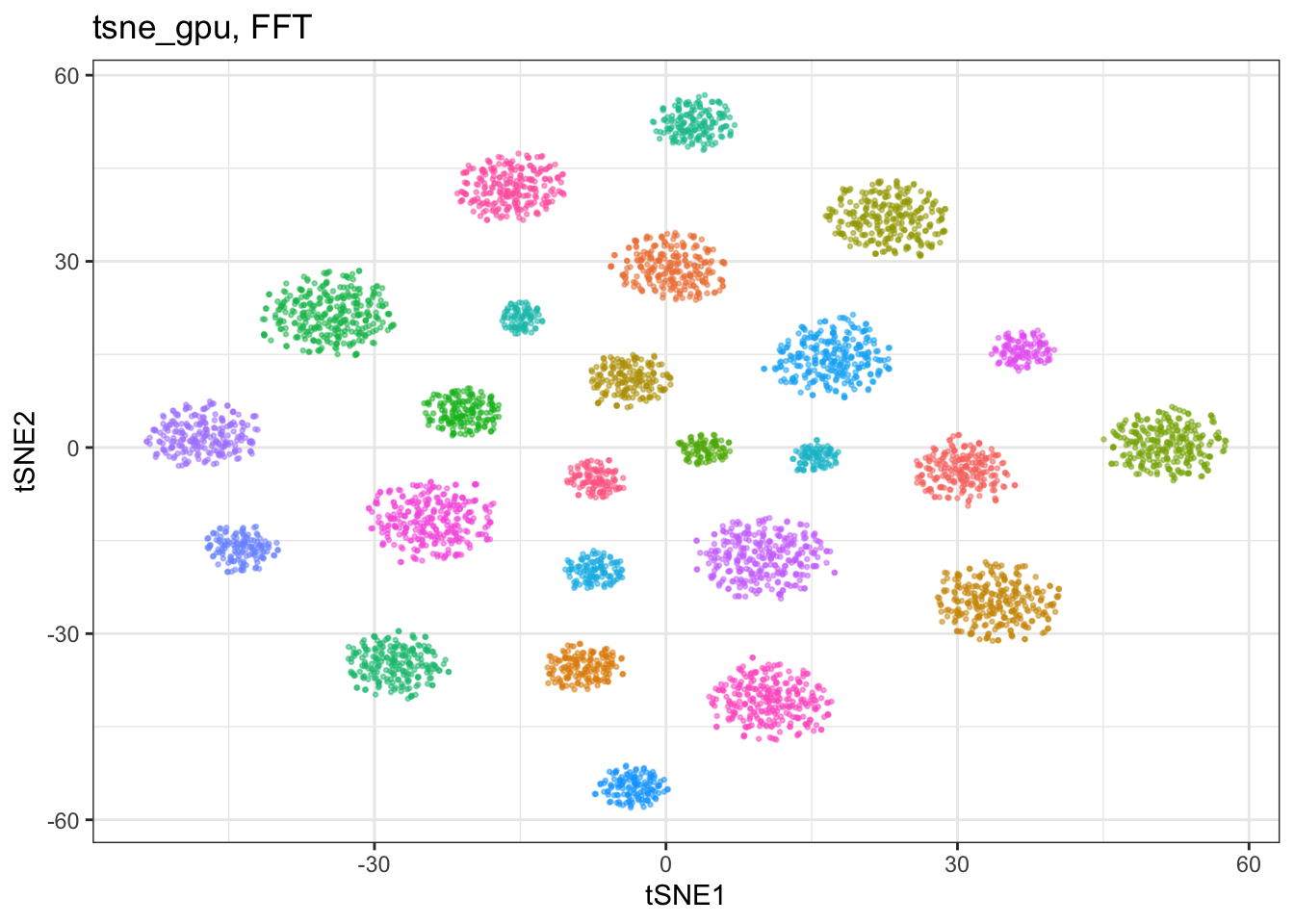
If you see the FFT embedding relax into a gapless disc rather than distinct cluster islands on very large data, that’s the equilibrium at exaggeration = 1. Set late_exag_factor in params_tsne_gpu() to a value between 2 and 4 to pull the clusters apart. Same caveat as the manifoldsR vignette.
Using a pre-computed kNN graph
Sweeping t-SNE hyperparameters (perplexity, learning rate, exaggeration) is usually where you spend the most time. Cache the kNN once and hand it in.
knn_precomputed <- generate_knn_graph_gpu(
  data = cluster_data$data,
  k = 90L, # ~ 3 * perplexity for perplexity = 30
  knn_method = "exhaustive",
  .verbose = TRUE
)

tsne_from_knn <- tsne_gpu(
  data = cluster_data$data,
  knn = knn_precomputed,
  perplexity = 30,
  tsne_params = params_tsne_gpu(),
  seed = 42L,
  .verbose = TRUE
)
#> Using provided kNN graph.

plot_df_knn <- as.data.table(tsne_from_knn) |>
  setnames(c("tSNE1", "tSNE2"))
plot_df_knn[, cluster := as.factor(cluster_data$membership)]

ggplot(plot_df_knn, aes(x = tSNE1, y = tSNE2)) +
  geom_point(aes(colour = cluster), size = 0.5, alpha = 0.5) +
  theme_bw() +
  theme(legend.position = "none") +
  ggtitle("tsne_gpu, pre-computed kNN")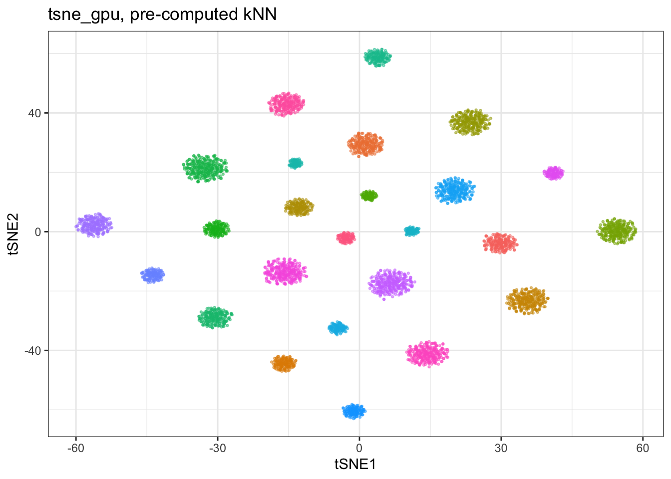
Note the kNN needs enough neighbours for the perplexity you’re using; k ≈ 3 * perplexity is the usual rule.
When does the GPU version pay off?
The CPU t-SNE in manifoldsR is already fast (Rust, SIMD kNN, FFT optimiser on Unix). The GPU version’s advantage is entirely in the kNN step, so the payoff depends on how much of your wall-clock the kNN eats. Generally speaking, if you have a larger data set, hit it with a GPU-accelerated kNN and the FFT optimiser. Longer term, the idea is to also implement 2D-FFT that is GPU-accelerated, but that is a larger project.
The kNN backend matters more here than in UMAP because the optimiser is still CPU either way. "nndescent" and "ivf" are the workhorses, "exhaustive" is for ground-truth checks or small data.
Conclusions
Same mental model as CPU t-SNE, same knobs, same caveats (t-SNE is a visualisation tool, cluster sizes and inter-cluster distances are not meaningful, see the manifoldsR vignette for the details). Current pipeline is hybrid: kNN on GPU, optimiser on CPU. Once the optimiser moves to GPU the whole thing runs on device end to end.