GPU-accelerated UMAP • bixverse.gpu

Intro

bixverse.gpu provides a GPU-accelerated UMAP via umap_gpu(). The surface mirrors the CPU version in manifoldsR, so if you’ve used that, you already know how to drive this. Kernels run on cubecl with the wgpu backend, so any compatible GPU works (including Apple Silicon).

Current split of work:

kNN graph construction: GPU. Three backends ("nndescent", "ivf", "exhaustive"), all GPU-accelerated.
Fuzzy simplicial set + init (spectral, PCA, or random): CPU. Porting these to GPU is on the roadmap.
Embedding optimisation: GPU. Adam on device (optimiser = "adam_gpu") is the default and usually the fastest.

The two heavy hitters (kNN, optimisation) run on the GPU, which is where most of the wall-clock sits for medium-to-large data. The CPU-side init and fuzzy-membership steps are comparatively cheap.

If you haven’t read the manifoldsR UMAP vignette, that one covers what UMAP is good at (cluster separation) and where it falls over (continuous manifolds). Both caveats apply here; only the compute path is different.

library(bixverse.gpu)
library(manifoldsR)
library(data.table)
#> Warning: package 'data.table' was built under R version 4.5.2
library(ggplot2)
#> Warning: package 'ggplot2' was built under R version 4.5.2

Note

Vignettes were built locally on a MacBook Pro M1 Max. The GH runners were just too slow and do not have proper GPU support. This gives an idea of speed on a decent, but older machine.

Generating data

Focus is on the case UMAP handles well: clustered data. 25k points across 25 clusters in 32D. Small enough to run fast, big enough that the GPU optimiser has something to chew on.

set.seed(42L)

cluster_data <- manifold_synthetic_data(
  type = "clusters",
  n_samples = 5000L,
  dim = 32L,
  parameters = params_clusters(n_clusters = 25L)
)

Running UMAP on GPU

Default call: NN-descent on GPU for kNN, spectral init on CPU, GPU Adam for the embedding.

umap_default <- umap_gpu(
  data = cluster_data$data,
  k = 15L,
  min_dist = 0.5,
  spread = 1.0,
  knn_method = "nndescent",
  umap_params = params_umap_gpu(),
  seed = 42L,
  .verbose = FALSE
)

plot_df <- as.data.table(umap_default) |>
  setnames(c("UMAP1", "UMAP2"))
plot_df[, cluster := as.factor(cluster_data$membership)]

ggplot(plot_df, aes(x = UMAP1, y = UMAP2)) +
  geom_point(aes(colour = cluster), size = 0.5, alpha = 0.5) +
  theme_bw() +
  theme(legend.position = "none") +
  ggtitle("umap_gpu, default (NN-descent + adam_gpu)")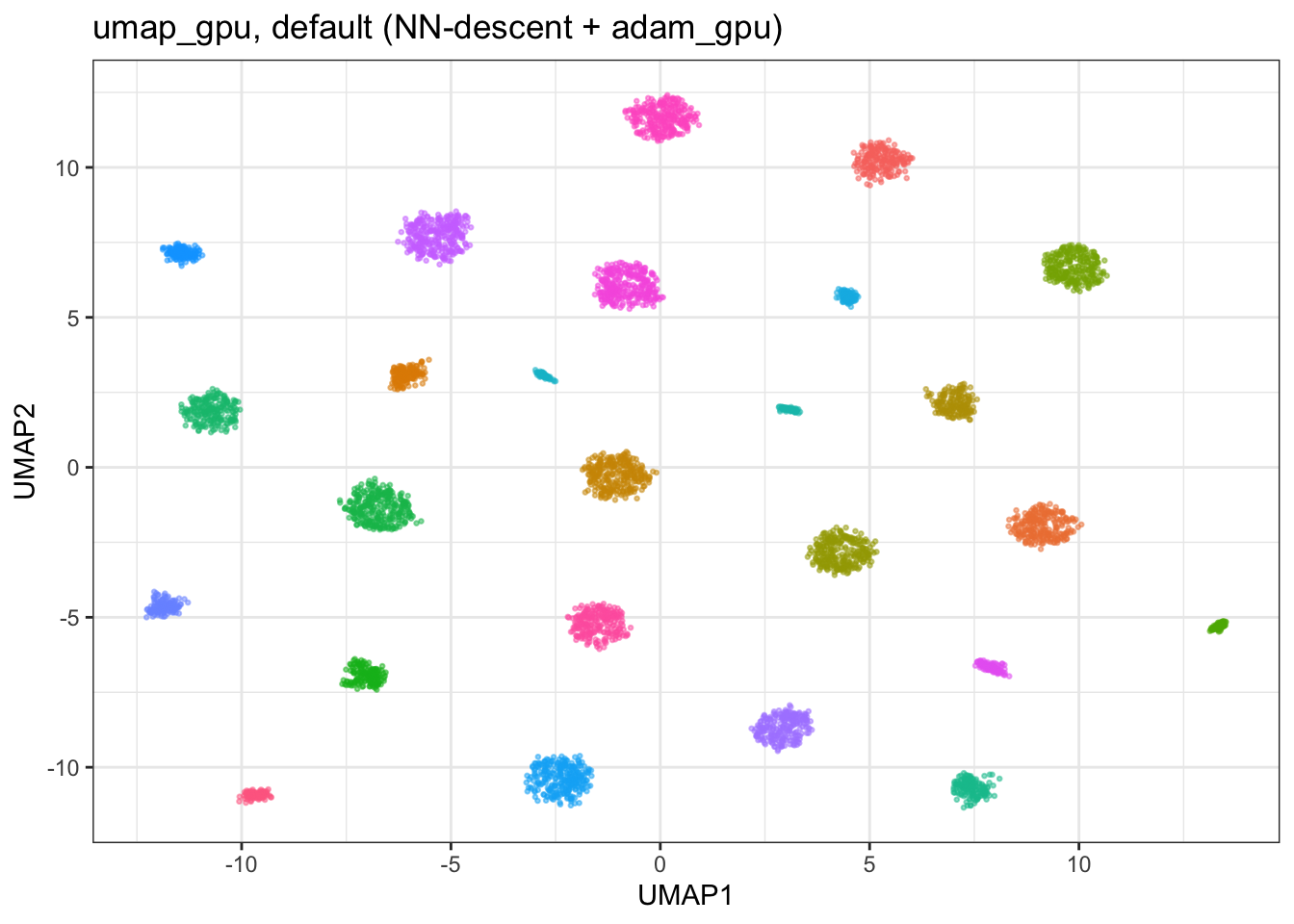

Clusters separate cleanly.

Choosing a kNN backend

Three GPU backends via knn_method:

"nndescent": NN-descent with CAGRA-style graph pruning. Solid default.
"ivf": inverted file index over Voronoi cells. Wins on large data where an approximate answer is fine.
"exhaustive": exact brute force. Small data or ground-truth checks. Quadratic in N, gets painful fast.

Tuning knobs live in params_nn_gpu(), defaults are fine for most cases.

IVF backend

umap_ivf <- umap_gpu(
  data = cluster_data$data,
  k = 15L,
  knn_method = "ivf",
  umap_params = params_umap_gpu(),
  seed = 42L,
  .verbose = FALSE
)

plot_df_ivf <- as.data.table(umap_ivf) |>
  setnames(c("UMAP1", "UMAP2"))
plot_df_ivf[, cluster := as.factor(cluster_data$membership)]

ggplot(plot_df_ivf, aes(x = UMAP1, y = UMAP2)) +
  geom_point(aes(colour = cluster), size = 0.5, alpha = 0.5) +
  theme_bw() +
  theme(legend.position = "none") +
  ggtitle("umap_gpu, IVF kNN")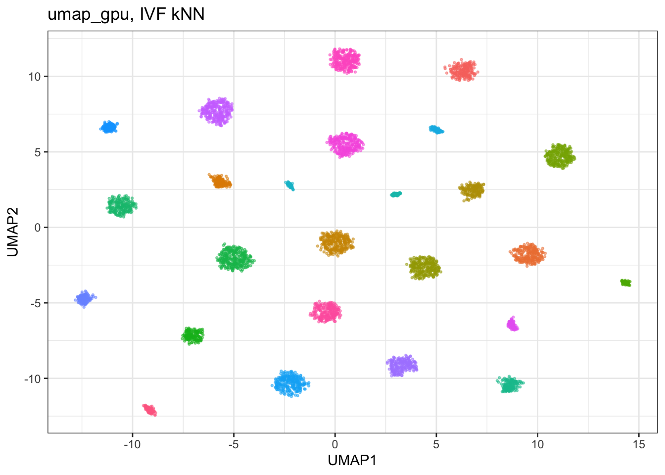

Exhaustive backend

umap_exhaustive <- umap_gpu(
  data = cluster_data$data,
  k = 15L,
  knn_method = "exhaustive",
  umap_params = params_umap_gpu(),
  seed = 42L,
  .verbose = FALSE
)

plot_df_ex <- as.data.table(umap_exhaustive) |>
  setnames(c("UMAP1", "UMAP2"))
plot_df_ex[, cluster := as.factor(cluster_data$membership)]

ggplot(plot_df_ex, aes(x = UMAP1, y = UMAP2)) +
  geom_point(aes(colour = cluster), size = 0.5, alpha = 0.5) +
  theme_bw() +
  theme(legend.position = "none") +
  ggtitle("umap_gpu, exhaustive kNN")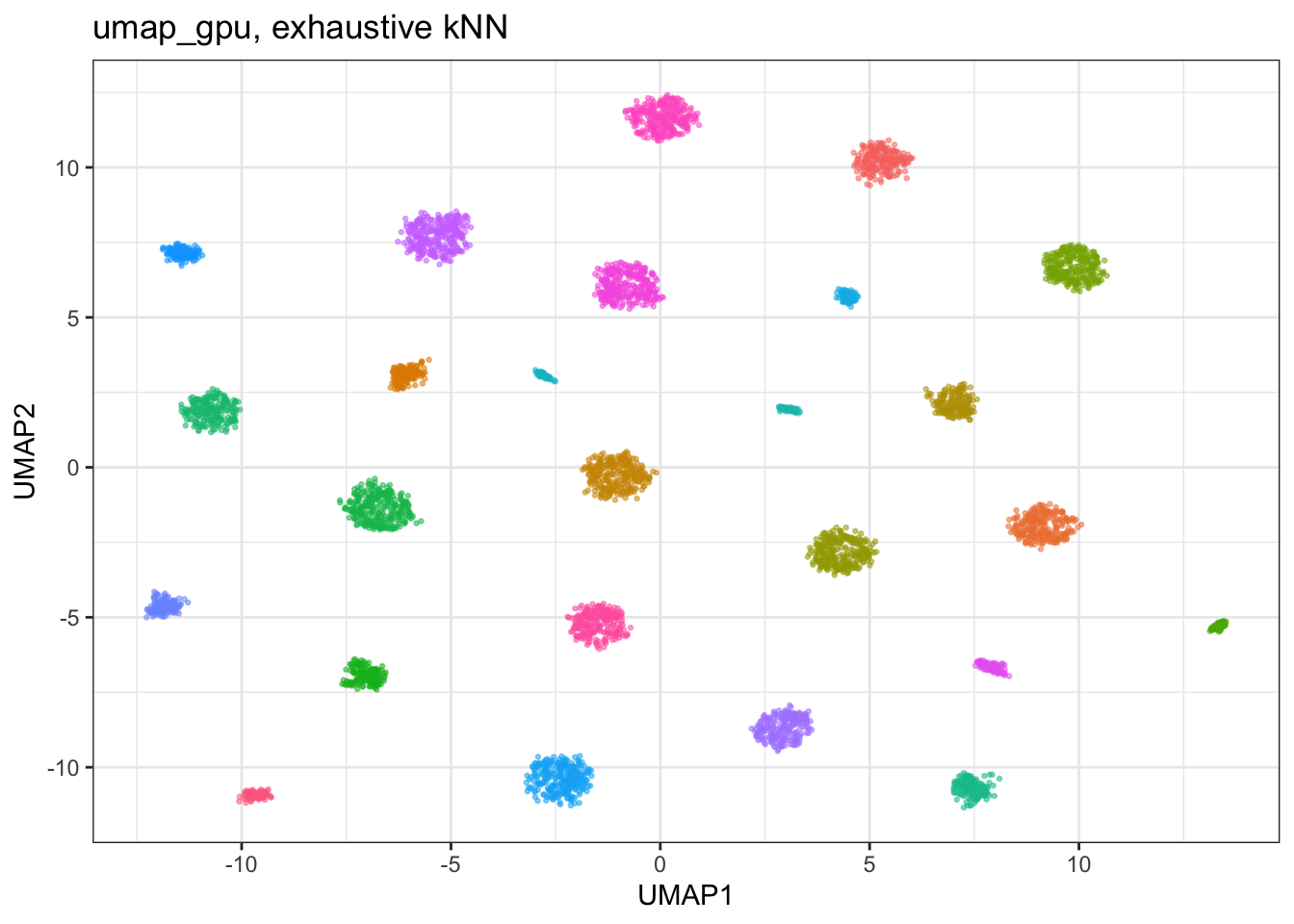

Structurally the three embeddings agree. Differences you see are within the noise of UMAP’s non-deterministic optimisation. The approximate methods are indistinguishable from exact for downstream analysis.

Choosing an optimiser

Four optimisers via params_umap_gpu(optimiser = ...):

"adam_gpu": GPU Adam, full optimisation on device with parallel gradient collection. Default, usually fastest.
"adam_parallel": CPU parallel Adam (the fast manifoldsR default). Handy if you want to keep the optimiser on CPU while still using the GPU kNN backend.
"adam": sequential CPU Adam. Can produce slightly cleaner embeddings on small data.
"sgd": classic stochastic gradient descent, as in the original UMAP paper. Slower, worth trying on continuous manifolds where you want a low min_dist to shine.

SGD optimiser

umap_sgd <- umap_gpu(
  data = cluster_data$data,
  k = 15L,
  min_dist = 0.3, # SGD prefers smaller min_dist
  knn_method = "nndescent",
  umap_params = params_umap_gpu(optimiser = "sgd"),
  seed = 42L,
  .verbose = FALSE
)

plot_df_sgd <- as.data.table(umap_sgd) |>
  setnames(c("UMAP1", "UMAP2"))
plot_df_sgd[, cluster := as.factor(cluster_data$membership)]

ggplot(plot_df_sgd, aes(x = UMAP1, y = UMAP2)) +
  geom_point(aes(colour = cluster), size = 0.5, alpha = 0.5) +
  theme_bw() +
  theme(legend.position = "none") +
  ggtitle("umap_gpu, SGD optimiser")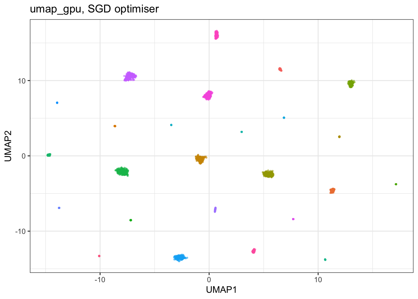

Parallel Adam optimiser

CPU parallel Adam (the manifoldsR::umap() default). Useful as a reference or when you want the optimiser on CPU and the kNN on GPU.

umap_ap <- umap_gpu(
  data = cluster_data$data,
  k = 15L,
  min_dist = 0.5,
  knn_method = "nndescent",
  umap_params = params_umap_gpu(optimiser = "adam_parallel"),
  seed = 42L,
  .verbose = FALSE
)

plot_df_ap <- as.data.table(umap_ap) |>
  setnames(c("UMAP1", "UMAP2"))
plot_df_ap[, cluster := as.factor(cluster_data$membership)]

ggplot(plot_df_ap, aes(x = UMAP1, y = UMAP2)) +
  geom_point(aes(colour = cluster), size = 0.5, alpha = 0.5) +
  theme_bw() +
  theme(legend.position = "none") +
  ggtitle("umap_gpu, adam_parallel optimiser")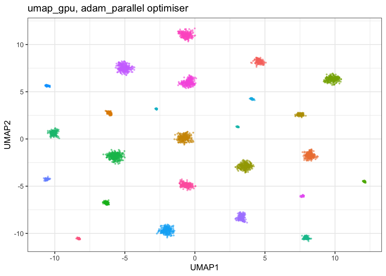

Using a pre-computed kNN graph

Already have a NearestNeighbours object (from manifoldsR or from one of the kNN routines in this package)? Hand it to umap_gpu() via the knn argument and skip the graph build. Handy when sweeping UMAP parameters.

knn_precomputed <- generate_knn_graph_gpu(
  data = cluster_data$data,
  k = 15L,
  .verbose = FALSE
)

umap_from_knn <- umap_gpu(
  data = cluster_data$data,
  knn = knn_precomputed,
  k = 15L,
  min_dist = 0.5,
  umap_params = params_umap_gpu(),
  seed = 42L,
  .verbose = FALSE
)

plot_df_knn <- as.data.table(umap_from_knn) |>
  setnames(c("UMAP1", "UMAP2"))
plot_df_knn[, cluster := as.factor(cluster_data$membership)]

ggplot(plot_df_knn, aes(x = UMAP1, y = UMAP2)) +
  geom_point(aes(colour = cluster), size = 0.5, alpha = 0.5) +
  theme_bw() +
  theme(legend.position = "none") +
  ggtitle("umap_gpu, pre-computed kNN")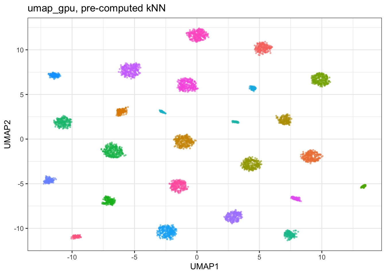

Sweeping min_dist is essentially free now; the expensive kNN build only runs once:

umap_wide <- umap_gpu(
  data = cluster_data$data,
  knn = knn_precomputed,
  k = 15L,
  min_dist = 1.0,
  umap_params = params_umap_gpu(),
  seed = 42L,
  .verbose = FALSE
)

plot_df_wide <- as.data.table(umap_wide) |>
  setnames(c("UMAP1", "UMAP2"))
plot_df_wide[, cluster := as.factor(cluster_data$membership)]

ggplot(plot_df_wide, aes(x = UMAP1, y = UMAP2)) +
  geom_point(aes(colour = cluster), size = 0.5, alpha = 0.5) +
  theme_bw() +
  theme(legend.position = "none") +
  ggtitle("umap_gpu, min_dist = 1.0")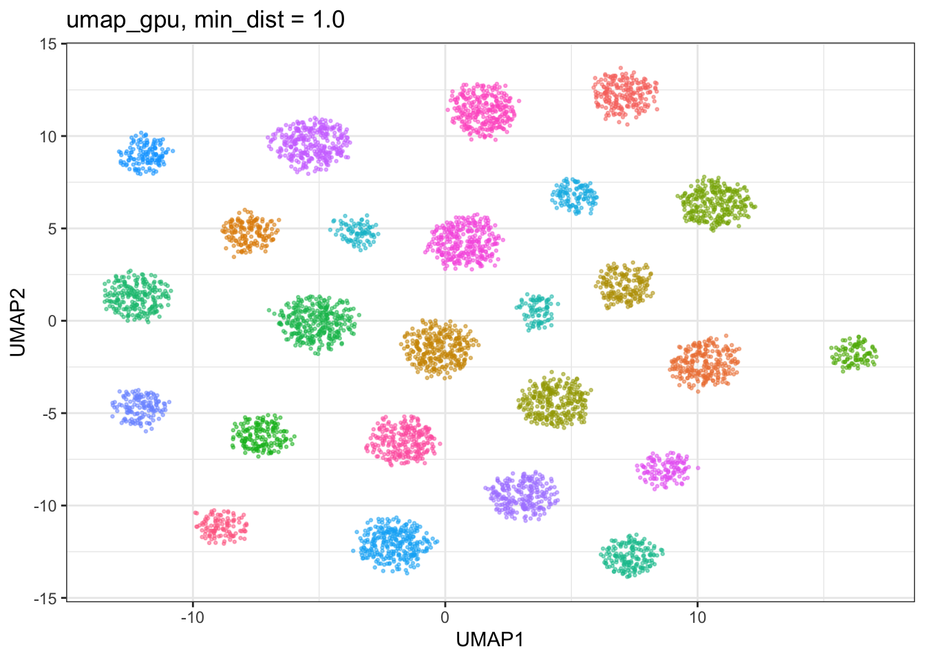

When does the GPU version pay off?

The CPU version in manifoldsR is already fast: parallel Adam, faer under the hood, full SIMD kNN toolkit. On Apple Silicon it’s especially competitive because wgpu doesn’t expose proper tensor-core equivalents on that hardware. On tall matrices with many samples the GPU optimiser and GPU kNN clearly pull ahead. On smaller data, kernel launch and host-device transfer overhead can wipe out the win.

Rough shape:

Below ~10k points: manifoldsR’s CPU parallel Adam is competitive or faster. GPU pays a fixed setup cost.
10k to 100k: GPU pulls ahead, especially with "ivf" or "nndescent".
Above 100k: GPU clearly faster, scales more gracefully with N.

Other axis is the kNN backend. "exhaustive" is quadratic in N, keep it for smaller data or ground-truth checks. "ivf" and "nndescent" are the workhorses.

Conclusions

Same mental model as CPU UMAP, same knobs, same caveats (UMAP is a visualisation tool, not a metric space!). Current pipeline is a hybrid: kNN and optimisation on GPU, fuzzy membership and init still on CPU. Both CPU steps are cheap and the GPU parts already deliver most of the speedup, but they’ll move to GPU eventually.

Downstream this ties into the single cell workflow: PCA on GPU, Harmony v2 on GPU, kNN on GPU, then UMAP on GPU. Minimum number of CPU handoffs in the reduce-embed-visualise chain.