Using t-SNE • manifoldsR

t-SNE in manifoldsR

manifoldsR provides a fast Rust-based implementation of t-SNE (t-Distributed Stochastic Neighbour Embedding), a widely used method for non-linear dimensionality reduction and visualisation. There is additionally the FFT-accelerated Interpolation-based t-SNE version available, based on the brilliant work of George, et al..

library(manifoldsR)
library(magrittr)
library(ggplot2)
library(data.table)

Intro

t-SNE works by modelling pairwise similarities between points in the high-dimensional space as a Gaussian distribution, and between points in the low-dimensional embedding as a Student t-distribution. It then minimises the Kullback-Leibler divergence between these two distributions via gradient descent. The heavy tails of the t-distribution are the key trick: they allow dissimilar points to be modelled far apart in the embedding without requiring enormous gradients, which alleviates the crowding problem that plagues earlier methods.

Compared to UMAP, t-SNE has a few notable properties worth keeping in mind:

Better at preserving local structure in continuous manifolds. Because the loss is symmetric and driven by pairwise probabilities rather than a graph connectivity objective, t-SNE tends to tear continuous structures apart less aggressively than UMAP. That said, it is not immune to this problem, particularly at low perplexity values.
Slower. The naive implementation is O(N^2), which quickly becomes prohibitive. The Barnes-Hut approximation ("bh") reduces this to O(N log N), and the FFT-accelerated version ("fft") further reduces it to O(N) — though the FFT variant is currently only supported on Unix systems due to cross-compilation constraints with FFTW.
No out-of-sample extension. Unlike UMAP, t-SNE embeddings cannot trivially be used to project new data points into the learned space. (To be fair, something that is not - yet - support in the package on the UMAP side.)
Distances within the embedding are not meaningful. Like UMAP, t-SNE is a visualisation tool. Cluster sizes and inter-cluster distances in the embedding should not be over-interpreted.

A key hyperparameter is perplexity, which loosely controls the effective number of neighbours each point considers. Typical values are between 5 and 50. Lower values focus on very local structure; higher values capture more global patterns. The learning rate and number of epochs also matter, particularly for large datasets.

Running t-SNE

We use the same synthetic datasets as in the UMAP vignette for direct comparison.

cluster_data <- manifold_synthetic_data(
  type = "cluster",
  n_samples = 25000L
)

swissrole_data <- manifold_synthetic_data(
  type = "swiss_role",
  n_samples = 1000L
)

trajectory_data <- manifold_synthetic_data(
  type = "trajectory",
  n_samples = 25000L
)

Clustered data

t-SNE is well known for producing crisp cluster separation. Let’s see how it handles the clustered synthetic data. But first, let’s check PCA…

pca_clusters <- prcomp(cluster_data$data)

pca_clusters_df <- as.data.table(pca_clusters$x[, 1:2]) %>%
  `colnames<-`(c("PC1", "PC2")) %>%
  .[, cluster := as.factor(cluster_data$membership)]

ggplot(
  data = pca_clusters_df,
  mapping = aes(x = PC1, y = PC2)
) +
  geom_point(mapping = aes(colour = cluster), size = 0.25, alpha = 0.5) +
  theme_bw() + 
  ggtitle("PCA on cluster data")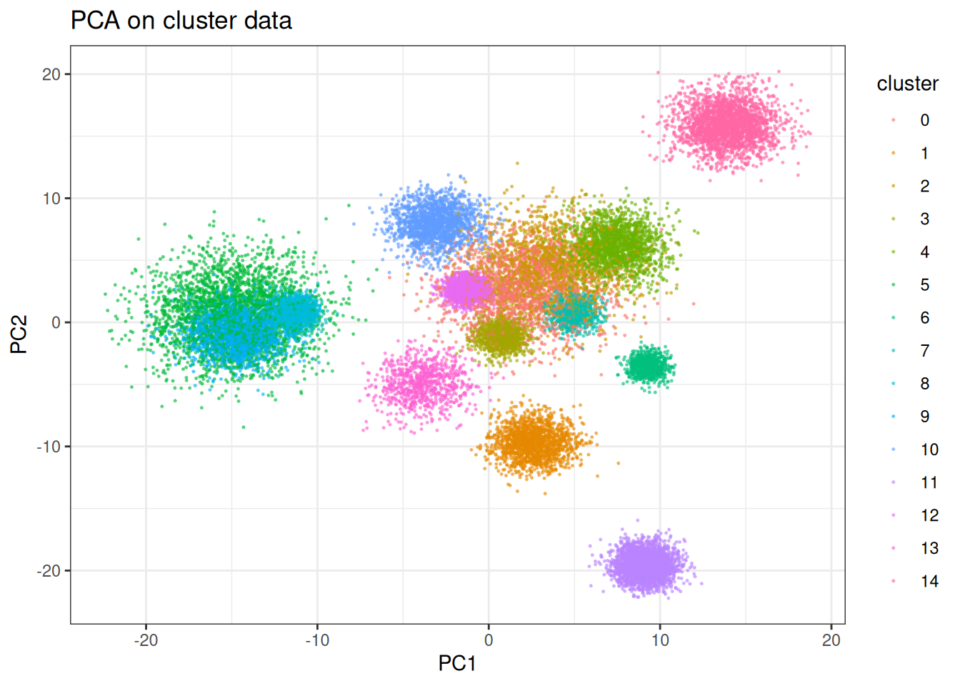

And now tSNE:

tsne_clusters <- tsne(
  data = cluster_data$data,
  perplexity = 30,
  seed = 42L
)

tsne_clustered_df <- as.data.table(tsne_clusters) %>%
  `colnames<-`(c("tSNE1", "tSNE2")) %>%
  .[, cluster := as.factor(cluster_data$membership)]

ggplot(
  data = tsne_clustered_df,
  mapping = aes(x = tSNE1, y = tSNE2)
) +
  geom_point(mapping = aes(colour = cluster), size = 0.25, alpha = 0.5) +
  theme_bw() + 
  ggtitle("tSNE (BH) on cluster data")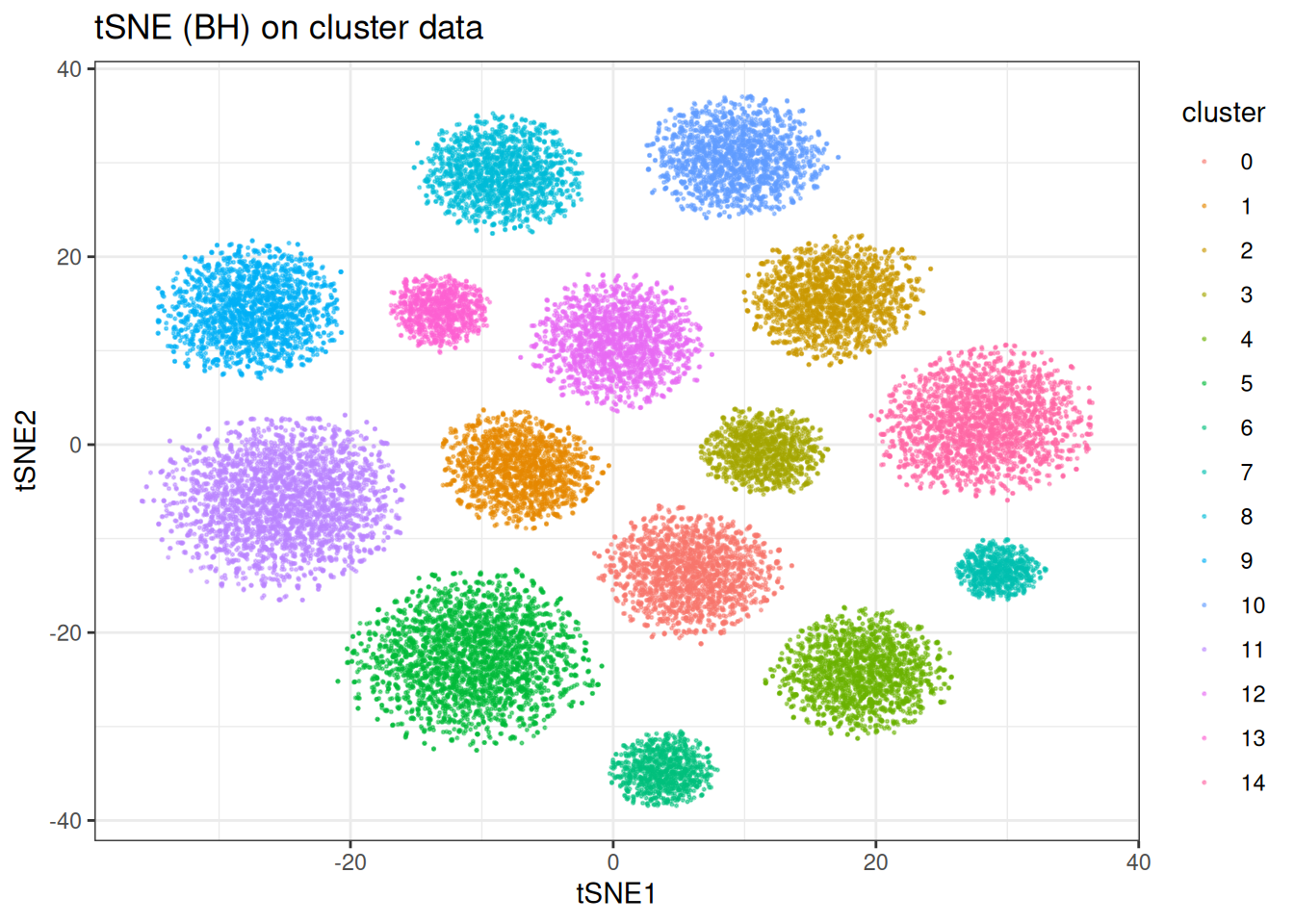

As expected, t-SNE separates the clusters cleanly. Worth noting: the inter-cluster distances and cluster sizes visible here are not directly interpretable — t-SNE optimises for local neighbourhood fidelity, not a faithful global geometry.

Swissrole

Let’s look at the swiss role, where UMAP struggled due to its graph-based objective. We will need higher perplexity values here to emphasise the global structure more. Similar to last UMAP, let’s start with PCA:

pca_swiss_role <- prcomp(swissrole_data$data)

pca_swiss_role_df <- as.data.table(pca_swiss_role$x[, 1:2]) %>%
  `colnames<-`(c("PC1", "PC2")) %>%
  .[, z_axis := swissrole_data$data[, 3]]

ggplot(
  data = pca_swiss_role_df,
  mapping = aes(x = PC1, y = PC2)
) +
  geom_point(
    mapping = aes(fill = z_axis), 
    shape = 21, 
    size = 2, 
    alpha = 0.5
  ) +
  scale_fill_viridis_c() +
  theme_bw() + 
  ggtitle("PCA on swissrole")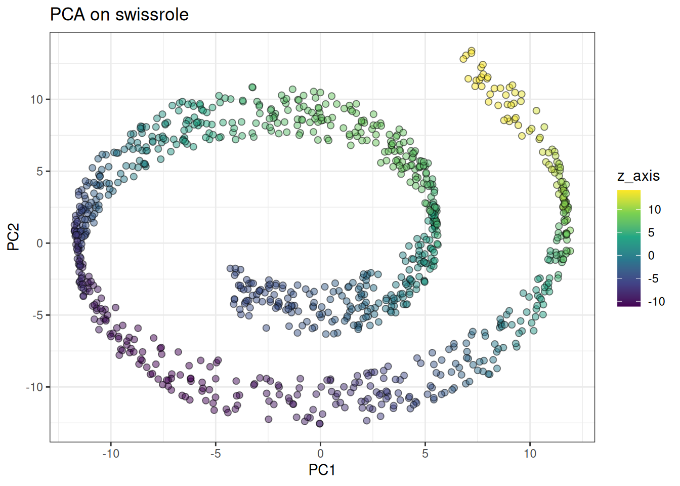

And compare against tSNE:

tsne_swissrole <- tsne(
  data = swissrole_data$data,
  knn_method = "exhaustive",
  perplexity = 50L, # we need to increase perplexity to capture the global structure
  seed = 42L
)

tsne_swissrole_df <- as.data.table(tsne_swissrole) %>%
  `colnames<-`(c("tSNE1", "tSNE2")) %>%
  .[, z_axis := swissrole_data$data[, 3]]

ggplot(
  data = tsne_swissrole_df,
  mapping = aes(x = tSNE1, y = tSNE2)
) +
  geom_point(
    mapping = aes(fill = z_axis),
    shape = 21,
    size = 2,
    alpha = 0.5
  ) +
  scale_fill_viridis_c() +
  theme_bw() + 
  ggtitle("tSNE (BH) on swissrole")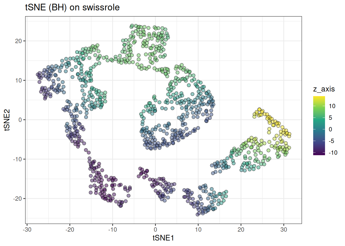

t-SNE handles the swiss role more gracefully than UMAP, preserving more of the continuous colour gradient along the roll. That said, it is still not perfect — this is still better approached with PCA or dedicated manifold unrolling methods (check out PHATE here).

Trajectory

Lastly, let’s look at trajectory type data…

pca_trajectory <- prcomp(trajectory_data$data)

pca_trajectory_df <- as.data.table(pca_trajectory$x[, 1:2]) %>%
  `colnames<-`(c("PC1", "PC2")) %>%
  .[, branch := trajectory_data$membership]

# will mix the labels to visualise the continuum better
ggplot(
  data = pca_trajectory_df[
    sample(1:nrow(pca_trajectory_df), nrow(pca_trajectory_df)), 
  ],
  mapping = aes(x = PC1, y = PC2)
) +
  geom_point(mapping = aes(colour = branch), alpha = 0.5, size = 0.25) +
  theme_bw() +
  scale_colour_viridis_c(option = "turbo") + 
  ggtitle("PCA on trajectory")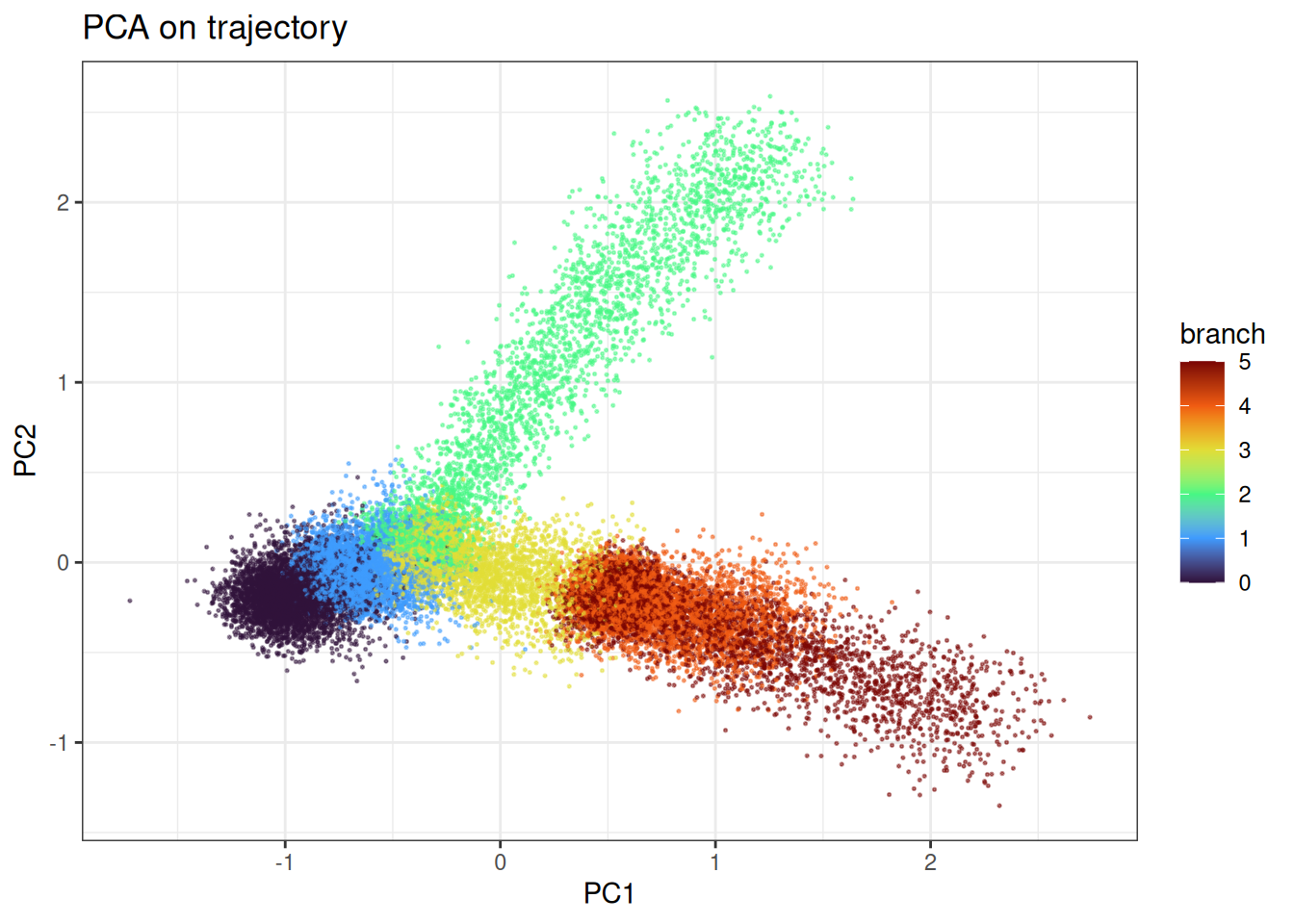

And tSNE

tsne_trajectory <- tsne(
  data = trajectory_data$data,
  perplexity = 45,
  seed = 42L
)

tsne_trajectory_df <- as.data.table(tsne_trajectory) %>%
  `colnames<-`(c("tSNE1", "tSNE2")) %>%
  .[, branch := trajectory_data$membership]

ggplot(
  data = tsne_trajectory_df[
    sample(1:nrow(tsne_trajectory_df), nrow(tsne_trajectory_df)),
  ],
  mapping = aes(x = tSNE1, y = tSNE2)
) +
  geom_point(
    mapping = aes(colour = branch),
    alpha = 0.5,
    size = 0.25
  ) +
  theme_bw() +
  scale_colour_viridis_c(option = "turbo") + 
  ggtitle("tSNE (BH) on trajectory")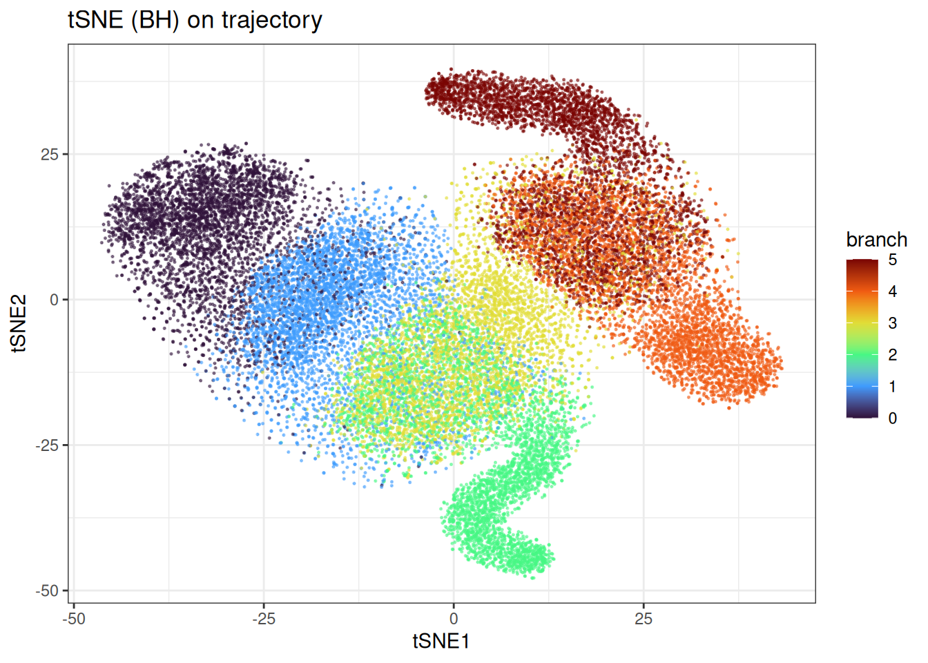

t-SNE does a better job of recovering the branching trajectory structure. Compared to UMAP, the continuous progression along each branch is somewhat better preserved, though the embedding still introduces distortions that are not present in a PCA plot and without knowing in detail how the differentiation path would go, it would not be clear.

Using pre-computed kNN graphs

If you want to test multiple parameter combinations while keeping the kNN graph fixed (e.g. varying perplexity or the number of epochs), you can precompute the kNN graph and pass it in directly.

precomputed_knn <- generate_knn_graph(
  data = cluster_data$data,
  k = 30L, # we will use 30 neighbours here...
  knn_method = "balltree",
  .verbose = FALSE
)

tsne_from_knn <- tsne(
  data = cluster_data$data,
  knn = precomputed_knn,
  perplexity = 30,
  seed = 42L
)
#> Using provided kNN graph.

tsne_from_knn_df <- as.data.table(tsne_from_knn) %>%
  `colnames<-`(c("tSNE1", "tSNE2")) %>%
  .[, cluster := as.factor(cluster_data$membership)]

ggplot(
  data = tsne_from_knn_df,
  mapping = aes(x = tSNE1, y = tSNE2)
) +
  geom_point(mapping = aes(colour = cluster), alpha = 0.5, size = 0.25) +
  theme_bw() +
  ggtitle("tSNE on pre-computed kNN (version 1)")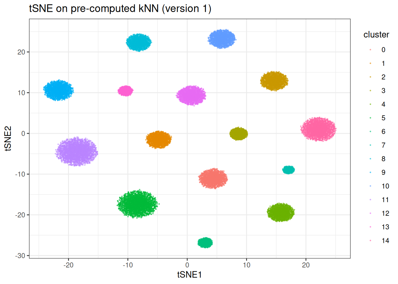

Now we can quickly re-run with different t-SNE parameters without repeating the kNN search:

tsne_from_knn_highperplex <- tsne(
  data = cluster_data$data,
  knn = precomputed_knn,
  perplexity = 100,
  tsne_params = params_tsne(n_epochs = 300L, lr = 100.0), # we will stop early to show a weirder embedding
  seed = 42L
)
#> Using provided kNN graph.

tsne_from_knn_highperplex_df <- as.data.table(tsne_from_knn_highperplex) %>%
  `colnames<-`(c("tSNE1", "tSNE2")) %>%
  .[, cluster := as.factor(cluster_data$membership)]

ggplot(
  data = tsne_from_knn_highperplex_df,
  mapping = aes(x = tSNE1, y = tSNE2)
) +
  geom_point(mapping = aes(colour = cluster), alpha = 0.5, size = 0.25) +
  theme_bw() +
  ggtitle("tSNE on pre-computed kNN (version 2)")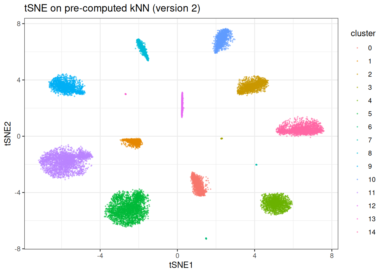

FFT-accelerated t-SNE

For large datasets, the Barnes-Hut approximation (O(N log N)) can still be slow. The FFT-accelerated variant reduces this to O(N) by interpolating the repulsive forces on a grid, making it substantially faster at scale. The constant however is higher. This version of tSNE becomes interesting in situations of ≥ 100,000 samples and more.

Note: the FFT variant is only available on Unix-based systems!

tsne_fft <- tsne(
  data = cluster_data$data,
  perplexity = 30,
  approx_type = "fft",
  seed = 42L
)

tsne_fft_df <- as.data.table(tsne_fft) %>%
  `colnames<-`(c("tSNE1", "tSNE2")) %>%
  .[, cluster := as.factor(cluster_data$membership)]

ggplot(
  data = tsne_fft_df,
  mapping = aes(x = tSNE1, y = tSNE2)
) +
  geom_point(mapping = aes(colour = cluster), alpha = 0.5, size = 0.25) +
  theme_bw()  + 
  ggtitle("tSNE (FFT) on cluster data")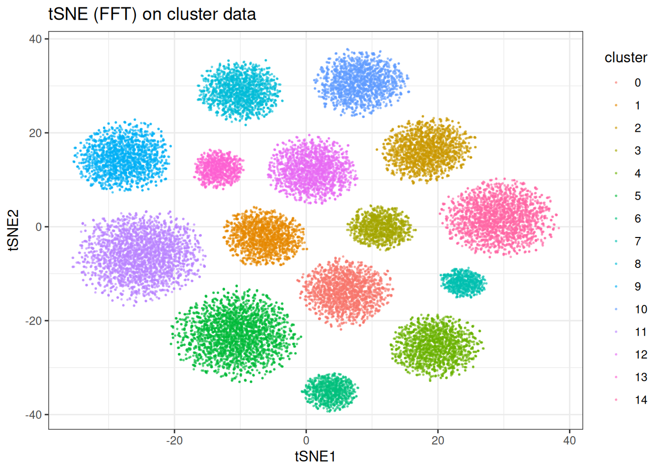

The embeddings are qualitatively similar to the BH version, with the FFT version trading a small amount of precision for a significant speed gain on large datasets.

Benchmarks

Let’s compare the BH implementation in manifoldsR against Rtsne (the most widely used t-SNE implementation in R, itself a wrapper around the C++ BH t-SNE code). The tsne package (pure R, naive O(N^2) implementation) is just too slow to be worth comparing here…

benchmark_data <- manifold_synthetic_data(
  type = "cluster",
  n_samples = 5000L
)

microbenchmark::microbenchmark(
  Rtsne = {
    Rtsne::Rtsne(
      X = benchmark_data$data,
      dims = 2,
      perplexity = 30,
      verbose = FALSE
    )
  },
  manifold_bh = {
    tsne(
      data = benchmark_data$data,
      perplexity = 30,
      approx_type = "bh",
      seed = 42L,
      .verbose = FALSE
    )
  },
  times = 1L
)
#> Unit: seconds
#>         expr       min        lq      mean    median        uq       max neval
#>        Rtsne 12.420229 12.420229 12.420229 12.420229 12.420229 12.420229     1
#>  manifold_bh  4.380563  4.380563  4.380563  4.380563  4.380563  4.380563     1

The impact here is massive already. Let’s see what happens with BH and FFT?

benchmark_data_large <- manifold_synthetic_data(
  type = "cluster",
  n_samples = 50000L 
)

microbenchmark::microbenchmark(
  manifold_bh = {
    tsne(
      data = benchmark_data_large$data,
      perplexity = 30,
      approx_type = "bh",
      seed = 42L,
      .verbose = FALSE
    )
  },
  manifold_fft = {
    tsne(
      data = benchmark_data_large$data,
      perplexity = 30,
      approx_type = "fft",
      seed = 42L,
      .verbose = FALSE
    )
  },
  times = 1L
)
#> Unit: seconds
#>          expr      min       lq     mean   median       uq      max neval
#>   manifold_bh 66.28111 66.28111 66.28111 66.28111 66.28111 66.28111     1
#>  manifold_fft 24.82410 24.82410 24.82410 24.82410 24.82410 24.82410     1

The speed advantage of the Rust implementation comes from a combination of optimised memory layout, aggressive inlining, and the fact that the entire pipeline — kNN construction, probability computation, and gradient descent — runs within the Rust kernel without round-tripping through R. If you like tSNE, but thought it’s too slow… we got you.