Using UMAP

Gregor Lueg

UMAP in manifoldsR

manifoldsR provides very rapid implementation of UMAP, based on the brilliant work in the uwot package. The aim of this version is to use a Rust-based version, R purely as an interface, and accelerate the algorithm even further.

library(manifoldsR)
library(magrittr)
library(ggplot2)
library(data.table)

Intro

UMAP works by constructing a weighted k-nearest neighbour graph in the high-dimensional space (see the knn_searches vignette for more details here!), where edge weights reflect the likelihood that two points are connected given their distance under a local, adaptive metric. Subsequently, It then minimises a cross-entropy loss between this high-dimensional graph and a low-dimensional analogue, effectively pulling connected nodes together and pushing unconnected ones apart. This objective is why UMAP excels at preserving cluster structure: if two points are unlikely neighbours in high dimensions, the repulsion term drives them apart in the embedding, producing clean separation. The flip side is that UMAP has no incentive to preserve the relative distances along a continuum. For trajectory or manifold data where the meaningful signal is a smooth progression, the loss treats weakly-connected distant points as things to repel rather than as part of a coherent structure. The result is that continuous manifolds tend to get torn apart into spurious clusters. Distances and even topology within an embedding should therefore be interpreted with caution — UMAP is a visualisation tool, not a metric space!.

Running UMAP

We are going to generate three different data sets to showcase the strengths (and weaknesses) of UMAP:

cluster_data <- manifold_synthetic_data(
  type = "cluster",
  n_samples = 25000L
)

swissrole_data <- manifold_synthetic_data(
  type = "swiss_role",
  n_samples = 1000L
)

trajectory_data <- manifold_synthetic_data(
  type = "trajectory",
  n_samples = 25000L
)

Clustered data

Let’s start with something UMAP does well - visualise well separated clusters. We will first contrast this against standard PCA to have some bases…

pca_clusters <- prcomp(cluster_data$data)

pca_clusters_df <- as.data.table(pca_clusters$x[, 1:2]) %>%
  `colnames<-`(c("PC1", "PC2")) %>%
  .[, cluster := as.factor(cluster_data$membership)]

ggplot(
  data = pca_clusters_df,
  mapping = aes(x = PC1, y = PC2)
) +
  geom_point(mapping = aes(colour = cluster), size = 0.25, alpha = 0.5) +
  theme_bw() +
  ggtitle("PCA on clustered data")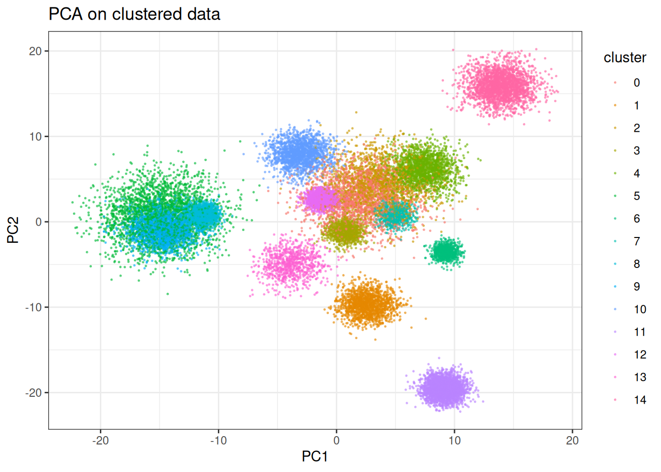

PCA does an okay job here; however, several of the clusters are clearly mixed. The separation likely occurs with different combination of the PCs, but let’s see what UMAP can do here on just two dimensions. We will start using the traditional stochastic gradient descent approach like in the original work and look at other (faster) optimisers later.

umap_clusters <- umap(
  data = cluster_data$data,
  min_dist = 0.3, # for sgd lower min dist is usually better
  umap_params = params_umap(optimiser = "sgd"),
  k = 15L
)
#> Using n_epochs = 200 (dataset <=10k samples with sgd/adam optimiser)

umap_clustered_df <- as.data.table(umap_clusters) %>%
  `colnames<-`(c("UMAP1", "UMAP2")) %>%
  .[, cluster := as.factor(cluster_data$membership)]

ggplot(
  data = umap_clustered_df,
  mapping = aes(x = UMAP1, y = UMAP2)
) +
  geom_point(mapping = aes(colour = cluster), alpha = 0.5, size = 0.25) +
  theme_bw() +
  ggtitle("UMAP (SGD) on clustered data")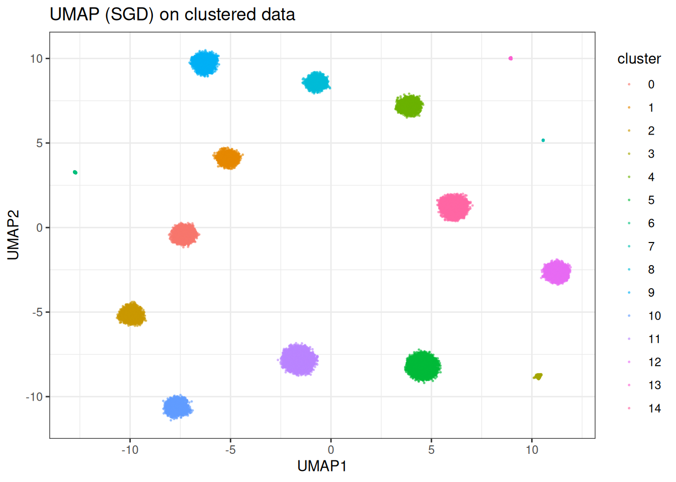

In this case, UMAP is clearly able to separate out the individual clusters (as expected). However, in other cases, UMAP does worse… Let’s look at the SwissRole example.

Swissrole

pca_swiss_role <- prcomp(swissrole_data$data)

pca_swiss_role_df <- as.data.table(pca_swiss_role$x[, 1:2]) %>%
  `colnames<-`(c("PC1", "PC2")) %>%
  .[, z_axis := swissrole_data$data[, 3]]

ggplot(
  data = pca_swiss_role_df,
  mapping = aes(x = PC1, y = PC2)
) +
  geom_point(
    mapping = aes(fill = z_axis), 
    shape = 21, 
    size = 2, 
    alpha = 0.5
  ) +
  scale_fill_viridis_c() +
  theme_bw() +
  ggtitle("PCA on swissrole")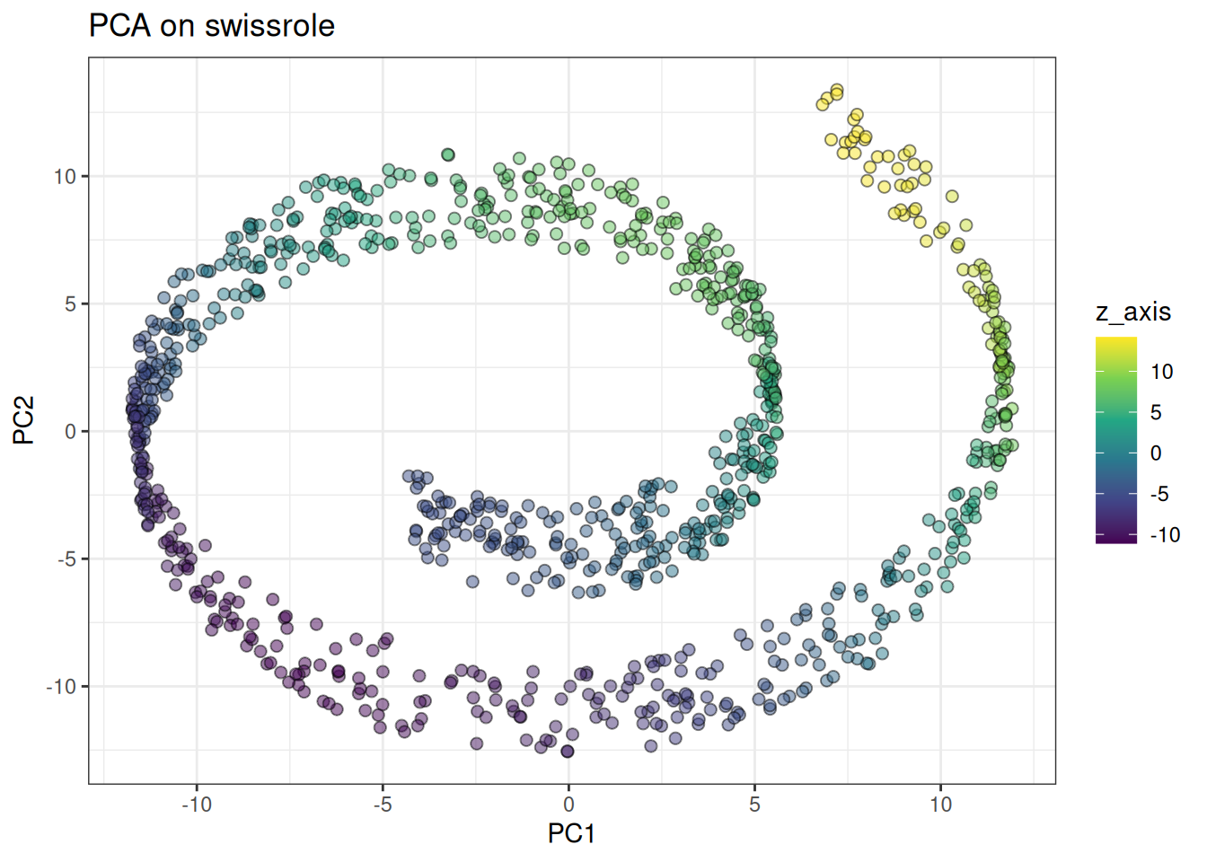

PCA clearly captures the Swissrole structure. How does UMAP perform here … ?

umap_swissrole <- umap(
  data = swissrole_data$data,
  knn_method = "exhaustive",
  min_dist = 0.3,
  umap_params = params_umap(optimiser = "sgd"),
  k = 10L # reduced because smaller
)
#> Using n_epochs = 500 (dataset <10k samples or adam_parallel optimiser)

umap_swissrole_df <- as.data.table(umap_swissrole) %>%
  `colnames<-`(c("UMAP1", "UMAP2")) %>%
  .[, z_axis := swissrole_data$data[, 3]]


ggplot(
  data = umap_swissrole_df,
  mapping = aes(x = UMAP1, y = UMAP2)
) +
  geom_point(
    mapping = aes(fill = z_axis), 
    shape = 21, 
    size = 2, 
    alpha = 0.5
  ) +
  scale_fill_viridis_c() +
  theme_bw() +
  ggtitle("UMAP on swissrole (SGD)")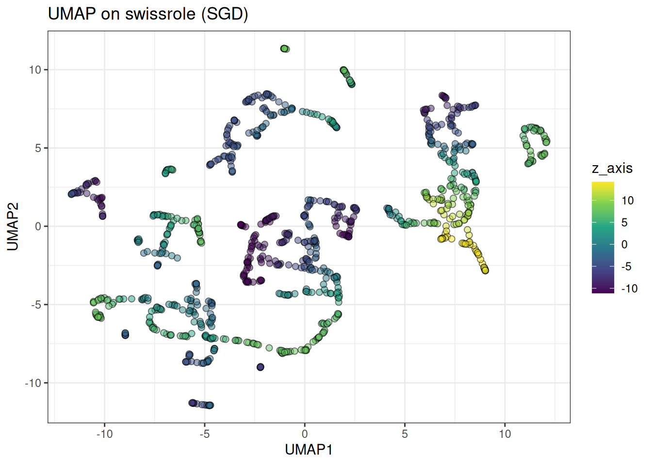

UMAP rips apart the swiss role structure. Due to the nature of the loss, it is not a great algorithm for data with a continuum-type manifold. This is also apparent in the trajectory type data, see below:

Trajectory

Let’s start with PCA again

pca_trajectory <- prcomp(trajectory_data$data)

pca_trajectory_df <- as.data.table(pca_trajectory$x[, 1:2]) %>%
  `colnames<-`(c("PC1", "PC2")) %>%
  .[, branch := trajectory_data$membership]

# will mix the labels to visualise the continuum better
ggplot(
  data = pca_trajectory_df[
    sample(1:nrow(pca_trajectory_df), nrow(pca_trajectory_df)), 
  ],
  mapping = aes(x = PC1, y = PC2)
) +
  geom_point(mapping = aes(colour = branch), alpha = 0.5, size = 0.25) +
  theme_bw() +
  scale_colour_viridis_c(option = "turbo") +
  ggtitle("PCA on trajectory data")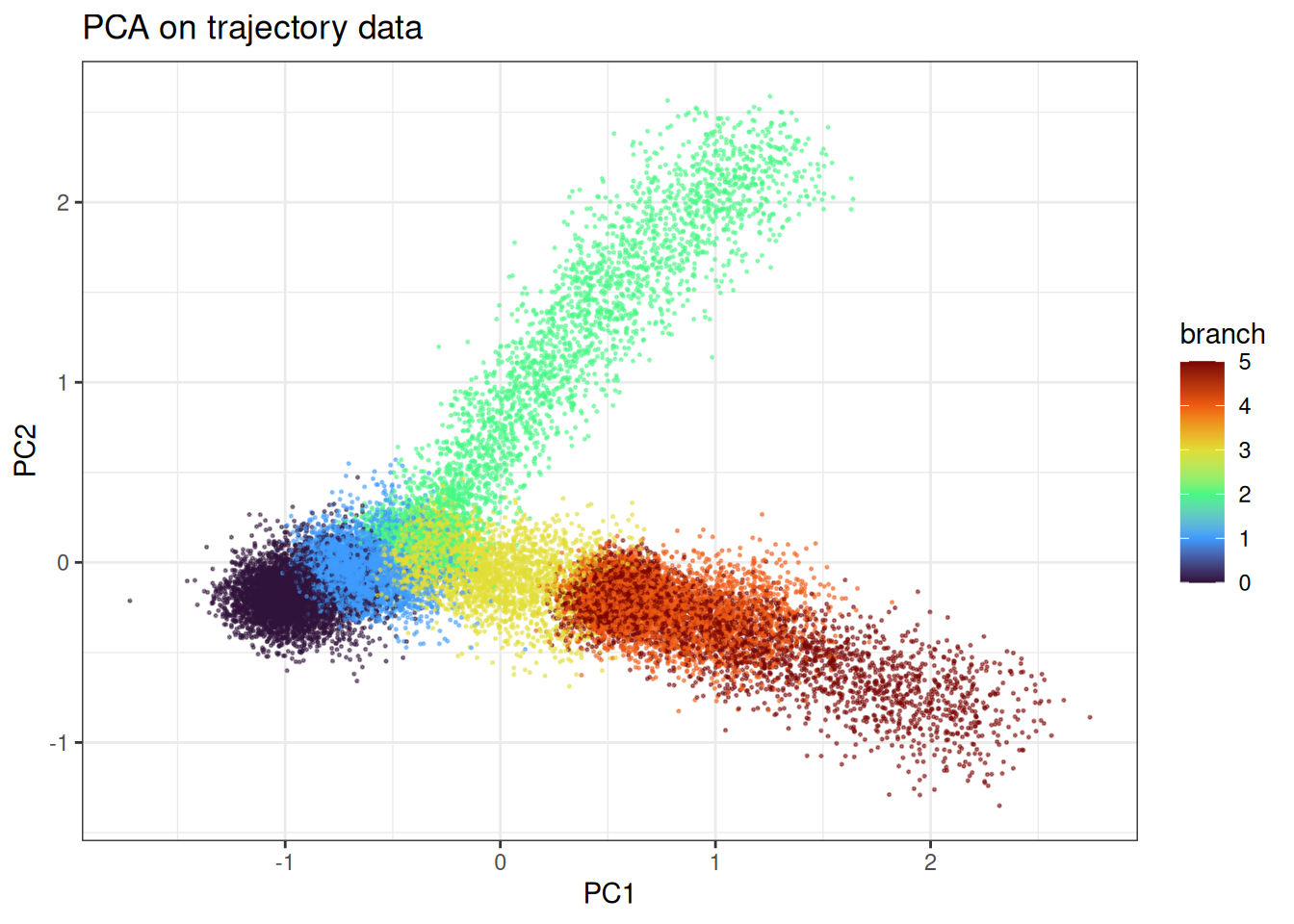

We can appreciate the branching and the continuum in the data.

umap_trajectory <- umap(
  data = trajectory_data$data,
  knn_method = "exhaustive",
  umap_params = params_umap(optimiser = "sgd"),
  min_dist = 0.3
)
#> Using n_epochs = 200 (dataset <=10k samples with sgd/adam optimiser)

umap_trajectory_df <- as.data.table(umap_trajectory) %>%
  `colnames<-`(c("UMAP1", "UMAP2")) %>%
  .[, branch := trajectory_data$membership]


ggplot(
  data = umap_trajectory_df[
    sample(1:nrow(pca_trajectory_df), nrow(pca_trajectory_df)), 
  ],
  mapping = aes(x = UMAP1, y = UMAP2)
) +
  geom_point(
    mapping = aes(colour = branch), 
    alpha = 0.5, 
    size = 0.25
  ) +
  theme_bw() +
  scale_colour_viridis_c(option = "turbo") +
  ggtitle("UMAP (SGD) on trajectory data")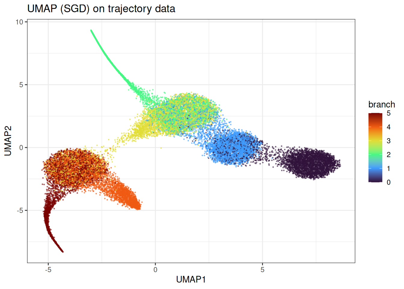

Here we observe the clear problem of UMAP. Instead of identifying the continuum in the manifold, we end up with more distinct clusters and some bleeding in between the clusters. However, this does not represent at all the underlying data.

Using pre-computed kNN parameters

As you have a range of parameters you might wish to test (while keeping the number of neighbours constant), you can also provide the NearestNeighbour class to the algorithm, see below:

precomputed_knn <- generate_knn_graph(
  data = cluster_data$data,
  k = 15L,
  knn_method = "balltree",
  .verbose = FALSE
)

umap_clusters_from_knn <- umap(
  data = cluster_data$data,
  knn = precomputed_knn,
  umap_params = params_umap(optimiser = "sgd"),
  k = 15L
)
#> Using n_epochs = 200 (dataset <=10k samples with sgd/adam optimiser)
#> Using provided kNN graph.

umap_clustered_from_knn_df <- as.data.table(umap_clusters_from_knn) %>%
  `colnames<-`(c("UMAP1", "UMAP2")) %>%
  .[, cluster := as.factor(cluster_data$membership)]

ggplot(
  data = umap_clustered_from_knn_df,
  mapping = aes(x = UMAP1, y = UMAP2)
) +
  geom_point(mapping = aes(colour = cluster), alpha = 0.5, size = 0.25) +
  theme_bw() +
  ggtitle("UMAP on pre-computed kNN")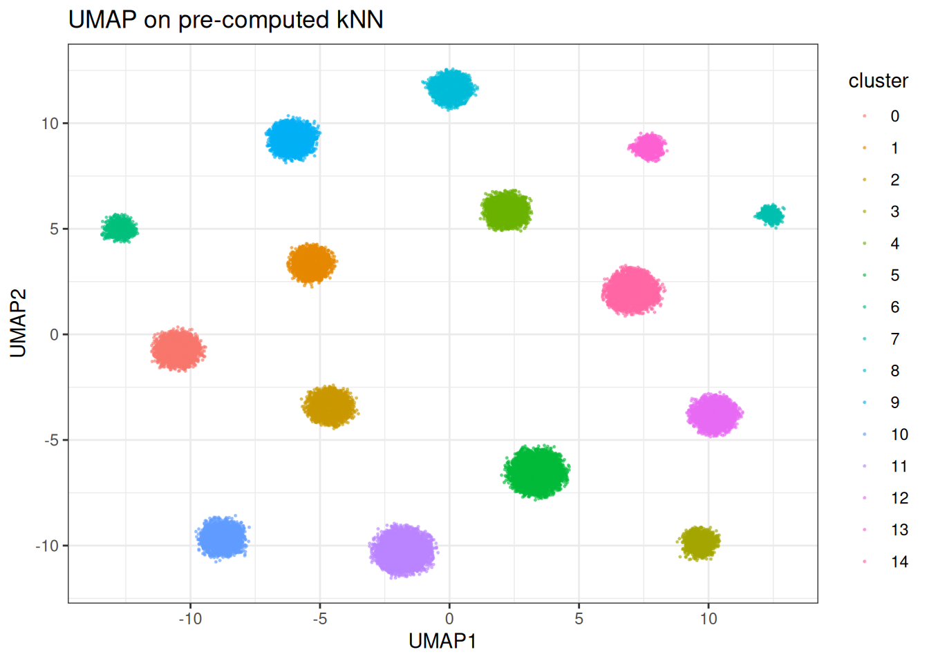

Let’s run quickly with different parameters

umap_clusters_from_knn <- umap(
  data = cluster_data$data,
  knn = precomputed_knn,
  min_dist = 1.0, # let's make the min_dist bigger
  umap_params = params_umap(optimiser = "sgd"),
  k = 15L
)
#> Using n_epochs = 200 (dataset <=10k samples with sgd/adam optimiser)
#> Using provided kNN graph.

umap_clustered_from_knn_df <- as.data.table(umap_clusters_from_knn) %>%
  `colnames<-`(c("UMAP1", "UMAP2")) %>%
  .[, cluster := as.factor(cluster_data$membership)]

ggplot(
  data = umap_clustered_from_knn_df,
  mapping = aes(x = UMAP1, y = UMAP2)
) +
  geom_point(mapping = aes(colour = cluster), alpha = 0.5, size = 0.25) +
  theme_bw()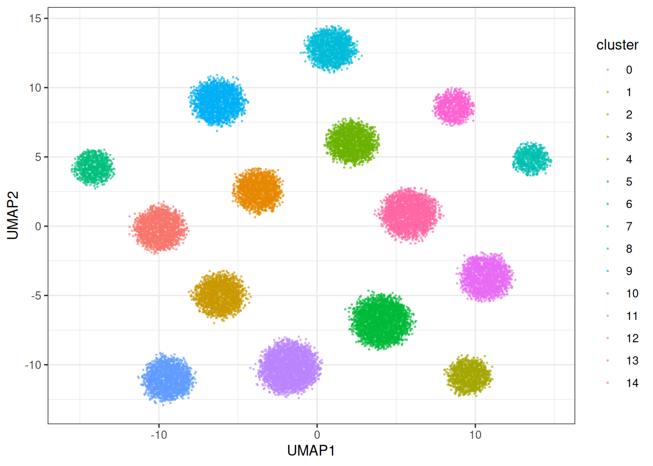

UMAP speed and optimisers

The package provides several optimisers with one of them designed for speed, i.e., the parallelised ADAM optimiser. This one is designed to deal with LARGE data sets you throw at the problem and it can generate the embeddings very fast. Let’s check out the other optimisers:

umap_clusters <- umap(
  data = cluster_data$data,
  umap_params = params_umap(optimiser = "adam")
)
#> Using n_epochs = 200 (dataset <=10k samples with sgd/adam optimiser)

umap_clustered_df <- as.data.table(umap_clusters) %>%
  `colnames<-`(c("UMAP1", "UMAP2")) %>%
  .[, cluster := as.factor(cluster_data$membership)]

ggplot(
  data = umap_clustered_df,
  mapping = aes(x = UMAP1, y = UMAP2)
) +
  geom_point(mapping = aes(colour = cluster), alpha = 0.5, size = 0.25) +
  theme_bw()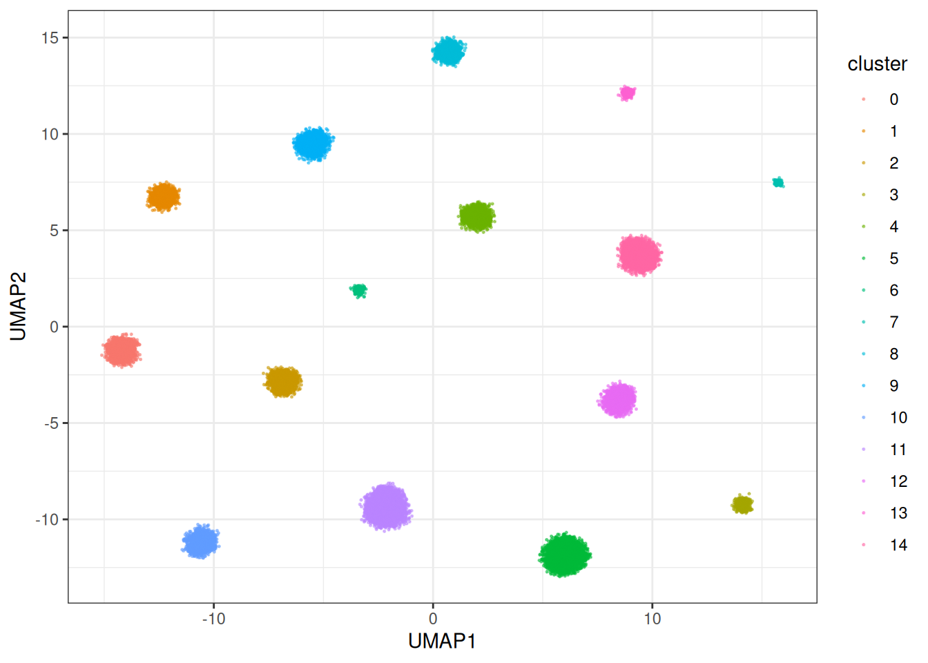

This one is actually a bit slower, but can in times generate nicer embeddings. But let’s look at the fast version… Parallised Adam (the default):

umap_clusters <- umap(
  data = cluster_data$data
)
#> Using n_epochs = 500 (dataset <10k samples or adam_parallel optimiser)

umap_clustered_df <- as.data.table(umap_clusters) %>%
  `colnames<-`(c("UMAP1", "UMAP2")) %>%
  .[, cluster := as.factor(cluster_data$membership)]


ggplot(
  data = umap_clustered_df,
  mapping = aes(x = UMAP1, y = UMAP2)
) +
  geom_point(
    mapping = aes(colour = cluster), 
    alpha = 0.5, 
    size = 0.25
  ) +
  theme_bw()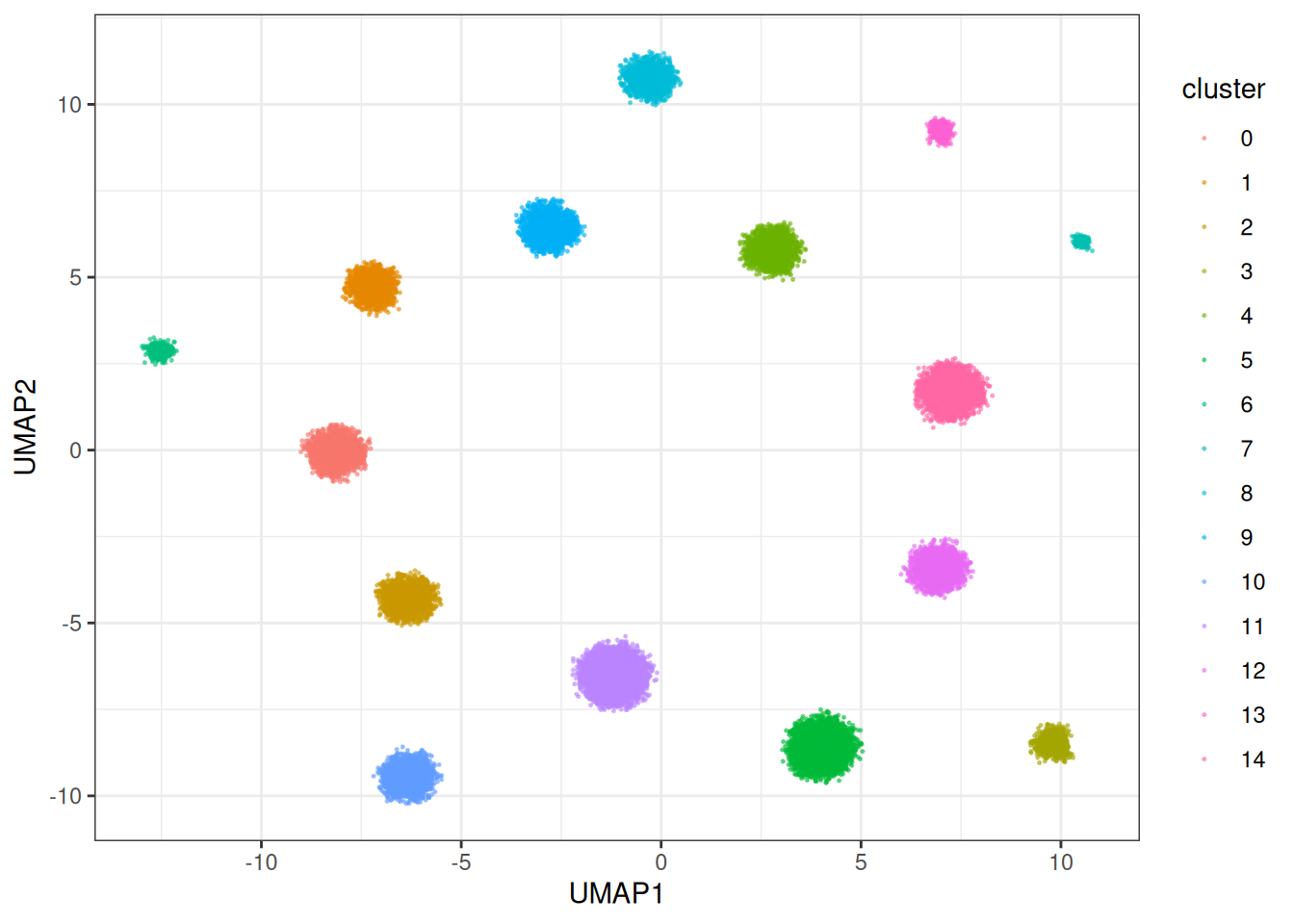

This one is SUBSTANTIALLY faster, as the gradients for each node in the graph are collected in parallel and then applied. This allows us to make usage of heavy multi-threading which Rust supports beautifully via Rayon. In terms of how does this version compare against other versions, let’s do a benchmark:

# set up the venv for the Python part/dependencies
local({
  env_name <- "r-manifolds"
  
  if (!reticulate::virtualenv_exists(env_name)) {
    reticulate::virtualenv_create(env_name)
    reticulate::virtualenv_install(
      env_name, 
      packages = c("phate", "umap-learn", "numpy", "scipy")
    )
  }
  
  if (!reticulate::py_available()) {
    reticulate::use_virtualenv(env_name, required = TRUE)
  }
  
  missing_pkgs <- Filter(
    Negate(reticulate::py_module_available),
    c("phate", "umap")
  )
  if (length(missing_pkgs) > 0L) {
    reticulate::virtualenv_install(
      env_name,
      packages = c("phate", "umap-learn", "numpy", "scipy")
    )
  }
})

benchmark_data <- manifold_synthetic_data(
  type = "cluster",
  n_samples = 5000L
)

umap_py <- reticulate::import("umap")

# initialise numba properly via JIT for fair comparison
# run a small dataset...
test_reducer <- umap_py$UMAP(
  n_neighbors = 15L, 
  n_jobs = parallel::detectCores() - 1L
)
test <- test_reducer$fit_transform(benchmark_data$data[1:500, ])

microbenchmark::microbenchmark(
  # umap version in pure R
  umap = {
    umap::umap(
      d = benchmark_data$data,
      method = "naive"
    )
  },
  umap_reticulate = {
    reducer <- umap_py$UMAP(
      n_neighbors = 15L,
      n_jobs = parallel::detectCores() - 1L
    )
    reducer$fit_transform(benchmark_data$data)
  },
  # uwot - umap, for example used in Seurat
  uwot = {
    uwot::umap(X = benchmark_data$data)
  },
  # uwot - umap2 version with parallel Adam under the hood
  # the approach that was also taken by manifoldsR
  uwot_v2 = {
    uwot::umap2(X = benchmark_data$data)
  },
  # the manifolds version
  manifold_umap = {
    umap(
      data = benchmark_data$data,
      k = 15L,
      .verbose = FALSE
    ) 
  },
  times = 1L # single comparison for speed
)
#> Unit: milliseconds
#>             expr        min         lq       mean     median         uq
#>             umap 20839.1114 20839.1114 20839.1114 20839.1114 20839.1114
#>  umap_reticulate 19629.6201 19629.6201 19629.6201 19629.6201 19629.6201
#>             uwot  4862.3332  4862.3332  4862.3332  4862.3332  4862.3332
#>          uwot_v2  3156.5036  3156.5036  3156.5036  3156.5036  3156.5036
#>    manifold_umap   588.2794   588.2794   588.2794   588.2794   588.2794
#>         max neval
#>  20839.1114     1
#>  19629.6201     1
#>   4862.3332     1
#>   3156.5036     1
#>    588.2794     1

We can appreciate that the standard R version is slow (as expected). If we leverage the Python version (with numba behind the scences) via the reticulate, we can get some speed ups (we need to however first JIT compile the numba parts). However, the uwot v2 version and the manifold are the fastest here. Let’s pit them together against each other in a larger data set.

benchmark_data_2 <- manifold_synthetic_data(
  type = "cluster",
  n_samples = 50000L
)

microbenchmark::microbenchmark(
  # uwot - umap2, for example used in Seurat
  uwot_v2 = {
    uwot::umap2(X = benchmark_data_2$data)
  },
  manifold_umap = {
    umap(
      data = benchmark_data_2$data,
      k = 15L,
      .verbose = FALSE
    ) 
  },
  times = 1L # single comparison for speed
)
#> Unit: seconds
#>           expr       min        lq      mean    median        uq       max
#>        uwot_v2 23.665031 23.665031 23.665031 23.665031 23.665031 23.665031
#>  manifold_umap  7.596204  7.596204  7.596204  7.596204  7.596204  7.596204
#>  neval
#>      1
#>      1

Due to optimised memory layouts, aggressive in-lining, heavy parallelism, leveragig look-up tables (LUTs), this version is fast and is likely(?) the fastest UMAP available in R, while keeping memory usage minimal due to leveraging Rust from the point that data is moved into the Rust kernel, until the embedding has been fitted. No round tripping through R, just highly optimised and compiled code throughout. The different nearest neighbour search algorithms give additional flexibility.