Metapath2vec
2026-09-24
Running metapath2vec
Setup
Background
Biological networks are rarely homogeneous. Genes interact with genes, genes sit in pathways, pathways sit in a hierarchy. Plain node2vec throws all of that into one pot and walks wherever the edges go. metapath2vec (Dong, Chawla and Swami) keeps the node types and forces every walk to follow a schema over them, a so-called metapath. gene-pathway-gene means: from a gene, hop to one of its pathways, then to another gene in that pathway, and repeat. The skip-gram model on top is the node2vec one; only the walks change.
Two things to know about the implementation:
- The walks are first-order. The next hop depends only on the current node and the position in the schema, so there’s no
pandq, and no(previous, current)transition table that blows up memory on dense graphs. -
metapath_plus = TRUEgives you metapath2vec++. Negative samples are then drawn from the context node’s own type, so a gene is contrasted against other genes and a pathway against other pathways.
Building a typed Reactome graph
The package ships a DuckDB with Reactome, and it has everything we need: gene to gene interactions, gene to pathway membership and the pathway hierarchy. We use two node types, gene and pathway.
gene_gene <- get_interactions_reactome()[, .(
  from = as.character(from),
  to = as.character(to)
)]
#> duckdb keeps downloaded extensions and secrets in a temporary directory:
#> ℹ /tmp/Rtmpm3wxlz/duckdb
#> This is removed when the R session ends.
#> • Extensions are re-downloaded each session.
#> • Secrets are lost.
#> ℹ Run duckdb(shared_home = TRUE) (or create ~/.duckdb) to keep them (suitable for most users).
#> ℹ Run duckdb(shared_home = FALSE) to accept the temporary directory (and silence this message).
#> ℹ See ?duckdb_storage for details and alternatives.
gene_pathway <- get_gene_to_reactome()[, .(
  from = as.character(from),
  to = as.character(to)
)]
#> duckdb keeps downloaded extensions and secrets in a temporary directory:
#> ℹ /tmp/Rtmpm3wxlz/duckdb
#> This is removed when the R session ends.
#> • Extensions are re-downloaded each session.
#> • Secrets are lost.
#> ℹ Run duckdb(shared_home = TRUE) (or create ~/.duckdb) to keep them (suitable for most users).
#> ℹ Run duckdb(shared_home = FALSE) to accept the temporary directory (and silence this message).
#> ℹ See ?duckdb_storage for details and alternatives.
pathway_pathway <- get_reactome_hierarchy("child_of")[, .(
  from = as.character(from),
  to = as.character(to)
)]
#> duckdb keeps downloaded extensions and secrets in a temporary directory:
#> ℹ /tmp/Rtmpm3wxlz/duckdb
#> This is removed when the R session ends.
#> • Extensions are re-downloaded each session.
#> • Secrets are lost.
#> ℹ Run duckdb(shared_home = TRUE) (or create ~/.duckdb) to keep them (suitable for most users).
#> ℹ Run duckdb(shared_home = FALSE) to accept the temporary directory (and silence this message).
#> ℹ See ?duckdb_storage for details and alternatives.

edges <- rbind(gene_gene, gene_pathway, pathway_pathway) %>%
  unique() %>%
  .[from != to]

nodes <- rbind(
  data.table(
    id = unique(c(gene_gene$from, gene_gene$to, gene_pathway$from)),
    type = "gene"
  ),
  data.table(
    id = unique(c(gene_pathway$to, pathway_pathway$from, pathway_pathway$to)),
    type = "pathway"
  )
) %>%
  unique(by = "id")

nodes[, .N, by = type]
#>       type     N
#>     <char> <int>
#> 1:    gene 11473
#> 2: pathway  2870
nrow(edges)
#> [1] 102292
metapath2vec wants two tables: the edges with from and to (and optionally weight), and the nodes with id and type. Every edge endpoint needs to be in the node table. For readable output later on, we also pull the gene symbols and pathway names.
node_labels <- rbind(
  get_gene_info()[, .(
    id = as.character(ensembl_id),
    label = as.character(symbol)
  )],
  get_reactome_info()[, .(
    id = as.character(reactome_id),
    label = as.character(reactome_name)
  )]
)
#> duckdb keeps downloaded extensions and secrets in a temporary directory:
#> ℹ /tmp/Rtmpm3wxlz/duckdb
#> This is removed when the R session ends.
#> • Extensions are re-downloaded each session.
#> • Secrets are lost.
#> ℹ Run duckdb(shared_home = TRUE) (or create ~/.duckdb) to keep them (suitable for most users).
#> ℹ Run duckdb(shared_home = FALSE) to accept the temporary directory (and silence this message).
#> ℹ See ?duckdb_storage for details and alternatives.
#> duckdb keeps downloaded extensions and secrets in a temporary directory:
#> ℹ /tmp/Rtmpm3wxlz/duckdb
#> This is removed when the R session ends.
#> • Extensions are re-downloaded each session.
#> • Secrets are lost.
#> ℹ Run duckdb(shared_home = TRUE) (or create ~/.duckdb) to keep them (suitable for most users).
#> ℹ Run duckdb(shared_home = FALSE) to accept the temporary directory (and silence this message).
#> ℹ See ?duckdb_storage for details and alternatives.
Check your walk statistics first
A schema that doesn’t fit the graph still gives you vectors. They’re just garbage. Every run records what happened during walk generation in the walk_stats attribute, so look at it! Here’s a schema that sounds sensible, from a gene to its pathway, up or down the hierarchy, and back to a gene:
bad_schema <- metapath2vec(
  graph_dt = edges,
  node_dt = nodes,
  metapath = c("gene", "pathway", "pathway", "gene"),
  metapath2vec_params = params_metapath2vec(
    walks_per_node = 5L,
    n_epochs = 1L
  ),
  .verbose = TRUE
)
#> Warning in metapath2vec(graph_dt = edges, node_dt = nodes, metapath = c("gene",
#> : Walks reach 15% of the requested length on average (6.0 of 40). The metapath
#> hits dead ends in the graph, check the schema.
#> 179 nodes were never visited by a walk and were removed.

bad_stats <- attr(bad_schema, "walk_stats")
str(bad_stats)
#> List of 6
#>  $ start_nodes: int 11473
#>  $ attempted  : int 57365
#>  $ truncated  : int 57152
#>  $ dropped    : int 85
#>  $ mean_length: num 6
#>  $ walk_length: int 40
99.6% of the walks dead-end before they reach the requested length, and the mean realised length is 6 instead of 40. Genes are mostly annotated to the leaves of the Reactome hierarchy, so the parent pathway you land on has no genes of its own to hop to. The schema is fine on paper; it just doesn’t match how this graph is wired.
Gene embeddings
gene-pathway-gene is the canonical choice. It ignores the interaction edges completely, so the embedding encodes shared pathway membership and nothing else. We run it as plain metapath2vec and as metapath2vec++, and add node2vec over the same edge table as the baseline.
walk_params <- params_metapath2vec(
  walks_per_node = 20L,
  walk_length = 40L,
  n_epochs = 10L
)

gpg <- metapath2vec(
  graph_dt = edges,
  node_dt = nodes,
  metapath = c("gene", "pathway", "gene"),
  embd_dim = 32L,
  metapath2vec_params = walk_params,
  .verbose = TRUE
)
#> 589 nodes were never visited by a walk and were removed.

str(attr(gpg, "walk_stats"))
#> List of 6
#>  $ start_nodes: int 11473
#>  $ attempted  : int 229460
#>  $ truncated  : int 340
#>  $ dropped    : int 340
#>  $ mean_length: num 41
#>  $ walk_length: int 41

gpg_plus <- metapath2vec(
  graph_dt = edges,
  node_dt = nodes,
  metapath = c("gene", "pathway", "gene"),
  embd_dim = 32L,
  metapath2vec_params = walk_params,
  metapath_plus = TRUE,
  .verbose = TRUE
)
#> 589 nodes were never visited by a walk and were removed.

n2v <- node2vec(
  graph_dt = edges,
  embd_dim = 32L,
  node2vec_params = params_node2vec(
    walks_per_node = 20L,
    walk_length = 40L,
    n_epochs = 10L
  ),
  .verbose = TRUE
)
This time the walk statistics look healthy: hardly any walk is truncated.
Do genes cluster by biology?
To score the embeddings, we need a label per gene. Reactome has 29 top-level pathways (signal transduction, metabolism, immune system, …). We walk the child_of edges up to them, and keep only the genes whose pathways all lead to a single top-level pathway, so the label is unambiguous.
parents <- pathway_pathway[, .(child = from, parent = to)]
roots <- setdiff(nodes[type == "pathway", id], parents$child)

# climb the hierarchy until every pathway has reached a root
ancestry <- data.table(pathway = nodes[type == "pathway", id])
ancestry[, top_level := pathway]
while (!all(ancestry$top_level %in% roots)) {
  ancestry <- merge(
    ancestry,
    parents,
    by.x = "top_level",
    by.y = "child",
    all.x = TRUE,
    allow.cartesian = TRUE
  ) %>%
    .[!is.na(parent), top_level := parent] %>%
    .[, parent := NULL] %>%
    unique()
}

gene_top_level <- merge(
  gene_pathway[, .(gene = from, pathway = to)],
  ancestry,
  by = "pathway"
)[, .(gene, top_level)] %>%
  unique()

gene_top_level <- gene_top_level[, if (.N == 1L) .SD, by = gene]

nrow(gene_top_level)
#> [1] 6542
The score is kNN purity: for each gene, the share of its 10 nearest neighbours (cosine) with the same top-level pathway. To keep this quick we sample 2,000 of the labelled genes.
knn_purity <- function(embd, labels, k = 10L) {
  x <- embd[labels$gene, ]
  x <- x / sqrt(rowSums(x^2))
  sim <- tcrossprod(x)
  diag(sim) <- -Inf
  nn <- t(apply(sim, 1, \(s) order(s, decreasing = TRUE)[seq_len(k)]))
  mean(matrix(labels$top_level[nn], ncol = k) == labels$top_level)
}

set.seed(42L)
eval_genes <- gene_top_level[sample(.N, 2000L)]

purity <- data.table(
  method = c(
    "node2vec",
    "metapath2vec (gene-pathway-gene)",
    "metapath2vec++ (gene-pathway-gene)",
    "random"
  ),
  knn_purity = c(
    knn_purity(n2v, eval_genes),
    knn_purity(gpg, eval_genes),
    knn_purity(gpg_plus, eval_genes),
    sum((eval_genes[, .N, by = top_level]$N / nrow(eval_genes))^2)
  )
)

purity
#>                                method knn_purity
#>                                <char>      <num>
#> 1:                           node2vec   0.783050
#> 2:   metapath2vec (gene-pathway-gene)   0.743600
#> 3: metapath2vec++ (gene-pathway-gene)   0.741950
#> 4:                             random   0.088955
All three are miles above random and within a few points of each other. The order shuffles between runs, since Hogwild training isn’t deterministic. That node2vec keeps up is no surprise: it sees the pathway edges as well, plus the interactions and the hierarchy, and the label is derived from the hierarchy. metapath2vec gets there from membership alone. metapath2vec++ barely moves the needle on this graph, since there are only two types and the gene side dominates the walks anyway. So what’s the point? You get to pick what “similar” means. With node2vec, you get whatever the graph mix gives you.
Nearest neighbours
Genes and pathways live in the same space, so we can ask one embedding for both. Here are the neighbours of TP53:
nearest <- function(embd, query, n = 10L) {
  x <- embd / sqrt(rowSums(embd^2))
  sim <- drop(x %*% x[query, ])
  top <- order(sim, decreasing = TRUE)[seq_len(n) + 1L]
  data.table(id = rownames(embd)[top], cosine = round(sim[top], 3)) %>%
    merge(nodes, by = "id", sort = FALSE) %>%
    merge(node_labels, by = "id", all.x = TRUE, sort = FALSE)
}

tp53 <- node_labels[label == "TP53", id][1]

nearest(gpg, tp53, n = 15L)
#>                  id cosine    type
#>              <char>  <num>  <char>
#>  1:   R-HSA-9723905  0.944 pathway
#>  2:     R-HSA-69895  0.872 pathway
#>  3:   R-HSA-6804754  0.849 pathway
#>  4:    R-HSA-111448  0.835 pathway
#>  5:   R-HSA-6804116  0.786 pathway
#>  6: ENSG00000161642  0.764    gene
#>  7:    R-HSA-139915  0.763 pathway
#>  8: ENSG00000104881  0.747    gene
#>  9: ENSG00000151615  0.747    gene
#> 10: ENSG00000152192  0.743    gene
#> 11: ENSG00000140836  0.737    gene
#> 12: ENSG00000165891  0.737    gene
#> 13: ENSG00000116017  0.736    gene
#> 14: ENSG00000129173  0.736    gene
#> 15: ENSG00000169372  0.735    gene
#>                                                                         label
#>                                                                        <char>
#>  1: Loss of function of TP53 in cancer due to loss of tetramerization ability
#>  2:                 Transcriptional  activation of  cell cycle inhibitor p21
#>  3:                                             Regulation of TP53 Expression
#>  4:                      Activation of NOXA and translocation to mitochondria
#>  5:    TP53 Regulates Transcription of Genes Involved in G1 Cell Cycle Arrest
#>  6:                                                                   ZNF385A
#>  7:                      Activation of PUMA and translocation to mitochondria
#>  8:                                                                  PPP1R13L
#>  9:                                                                    POU4F2
#> 10:                                                                    POU4F1
#> 11:                                                                     ZFHX3
#> 12:                                                                      E2F7
#> 13:                                                                    ARID3A
#> 14:                                                                      E2F8
#> 15:                                                                     CRADD
Pathway embeddings
Flip the schema to pathway-gene-pathway and the walks start on pathways. Two pathways end up close when they share genes, which is a smooth version of the Jaccard overlap you’d otherwise compute by hand. And it’s fast, because there are far fewer pathways than genes to start walks from.
pgp <- metapath2vec(
  graph_dt = edges,
  node_dt = nodes,
  metapath = c("pathway", "gene", "pathway"),
  embd_dim = 32L,
  metapath2vec_params = walk_params,
  .verbose = TRUE
)
#> Warning in metapath2vec(graph_dt = edges, node_dt = nodes, metapath =
#> c("pathway", : 19.9% of walks were dropped: their 'pathway' start node has no
#> 'gene' neighbour. Check the metapath against the graph.
#> 608 nodes were never visited by a walk and were removed.

str(attr(pgp, "walk_stats"))
#> List of 6
#>  $ start_nodes: int 2870
#>  $ attempted  : int 57400
#>  $ truncated  : int 11440
#>  $ dropped    : int 11440
#>  $ mean_length: num 41
#>  $ walk_length: int 41
About a fifth of the walks get dropped straight away. They start on the higher-level pathways with no directly annotated genes, same story as above. No walk ever touches those pathways, so all they’d have is their random initialisation. The same goes for genes with interactions only, since this schema never uses the gene-gene edges. metapath2vec() removes such nodes by default and lists them in the unvisited_nodes attribute (set filter_unvisited = FALSE if you want the rows anyway):
A pathway’s closest neighbours are its own member genes, so for pathway to pathway similarity we search the pathway rows only. Neighbours of TNFR1-induced proapoptotic signalling:
tnfr1 <- node_labels[label == "TNFR1-induced proapoptotic signaling", id][1]

nearest(pgp[pathway_ids, ], tnfr1)
#>                id cosine    type
#>            <char>  <num>  <char>
#>  1: R-HSA-5357956  0.923 pathway
#>  2: R-HSA-5357905  0.914 pathway
#>  3: R-HSA-9693928  0.900 pathway
#>  4: R-HSA-9686347  0.847 pathway
#>  5: R-HSA-5218900  0.844 pathway
#>  6: R-HSA-9013957  0.839 pathway
#>  7:  R-HSA-933543  0.838 pathway
#>  8: R-HSA-3371378  0.836 pathway
#>  9:   R-HSA-75157  0.829 pathway
#> 10:   R-HSA-69416  0.822 pathway
#>                                                                         label
#>                                                                        <char>
#>  1:                                TNFR1-induced NF-kappa-B signaling pathway
#>  2:                                             Regulation of TNFR1 signaling
#>  3:                               Defective RIPK1-mediated regulated necrosis
#>  4:                 Microbial modulation of RIPK1-mediated regulated necrosis
#>  5:                                               CASP8 activity is inhibited
#>  6:                      TLR3-mediated TICAM1-dependent programmed cell death
#>  7: NF-kB activation through FADD/RIP-1 pathway mediated by caspase-8 and -10
#>  8:                                                      Regulation by c-FLIP
#>  9:                                                     FasL/ CD95L signaling
#> 10:                                              Dimerization of procaspase-8
A PCA over the pathway rows, coloured by the eight largest top-level pathways:
pca_results <- prcomp(pgp[pathway_ids, ])

top_levels <- ancestry[, .N, by = top_level][order(-N)][1:8, top_level]

pca_dt <- as.data.table(pca_results$x[, 1:2], keep.rownames = "pathway") %>%
  merge(ancestry, by = "pathway") %>%
  .[, if (.N == 1L) .SD, by = pathway] %>%
  .[top_level %in% top_levels] %>%
  merge(
    node_labels[, .(top_level = id, top_level_name = label)],
    by = "top_level"
  )

ggplot(data = pca_dt, mapping = aes(x = PC1, y = PC2)) +
  geom_point(
    mapping = aes(fill = top_level_name),
    size = 2,
    alpha = 0.7,
    shape = 21,
    stroke = 0.2
  ) +
  theme_bw() +
  labs(fill = "Top-level pathway:") +
  scale_fill_viridis_d(option = "turbo")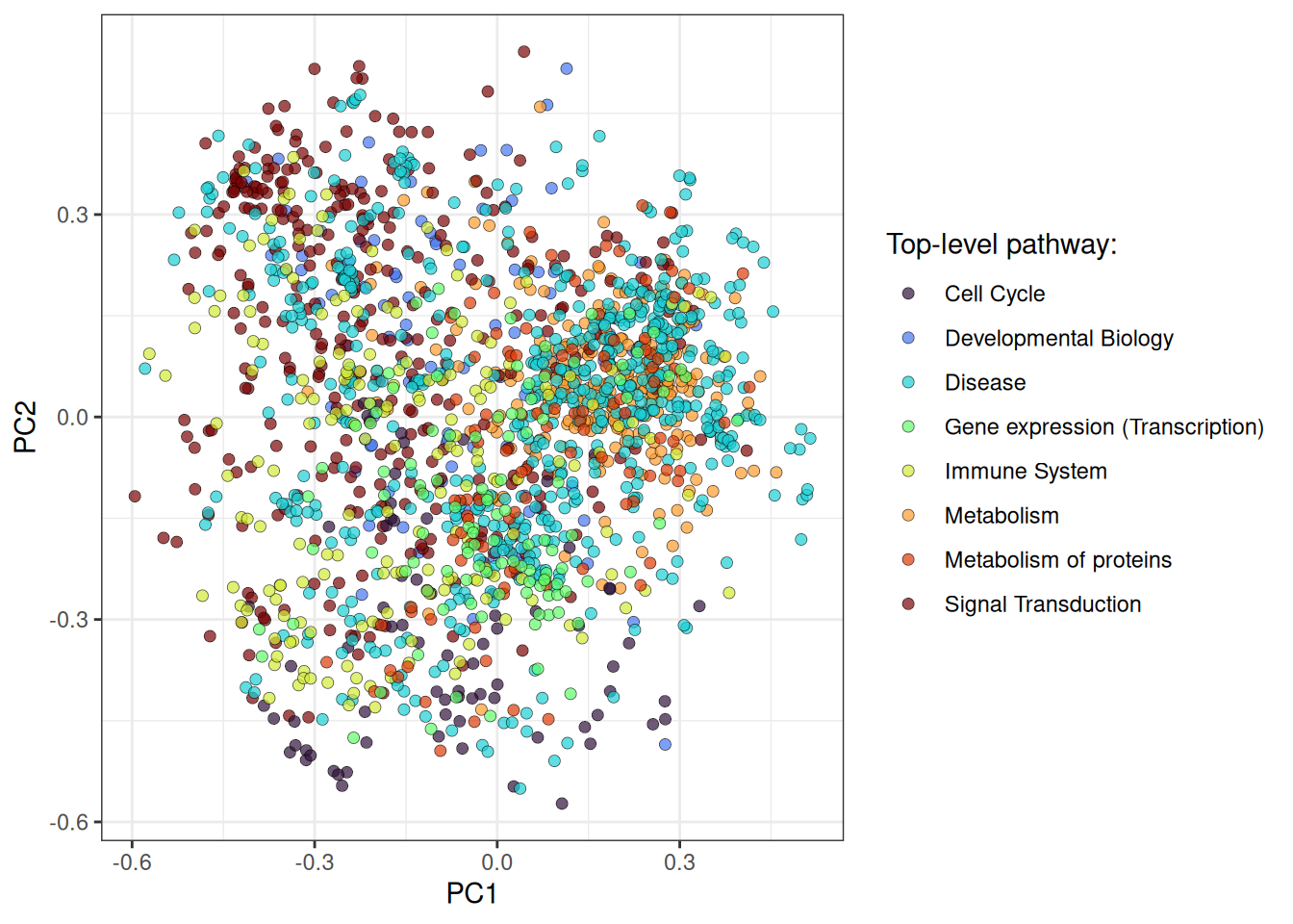
Two components out of 32 are a blunt view, but the broad layout is there: metabolism on one side, signal transduction on the other, immune system and developmental biology pulling apart along PC2. Disease is all over the place, which is fair: Reactome’s disease branch reuses the genes of every other branch.
Where to go from here
The walk engine takes up to 256 node types, so adding Gene Ontology as a third type is a table join away: gene-go-gene next to gene-pathway-gene gives you two views of function you can compare. On the roadmap: several metapaths in one run, which the original paper also discusses and which avoids having to pick a single schema up front.