library(manifoldsR)
library(magrittr)
library(ggplot2)
library(data.table)
#>
#> Attaching package: 'data.table'
#> The following object is masked from 'package:base':
#>
#> %notin%Using PHATE
2026-05-08
PHATE in manifoldsR
manifoldsR provides a fast Rust-based implementation of PHATE (Potential of Heat-diffusion for Affinity-based Trajectory Embedding), a dimensionality reduction method specifically designed for recovering continuous structure and trajectories in high-dimensional data.
Intro
PHATE builds an embedding through a sequence of steps. First, it constructs a kernel-based affinity graph over the data, using an adaptive bandwidth kernel controlled by the decay parameter. The kernel is then row-normalised to form a Markov transition matrix — i.e. a diffusion operator — which models random walks across the data manifold. Diffusion is run for t steps, either chosen automatically via Von Neumann entropy (up to t_max) or fixed via t_custom. Running diffusion for multiple steps has a denoising effect: local noise is smoothed out, and the global manifold geometry becomes more prominent.
From the diffused transition probabilities, PHATE computes a potential distance: it takes the log of the diffused probabilities and uses the difference between them as a geometrically meaningful distance metric. The gamma parameter controls the precise form of this transformation. Finally, MDS is applied to this potential distance matrix to produce the low-dimensional embedding.
Compared to t-SNE and UMAP, PHATE has a distinct character:
- Designed for continuous structure. PHATE was developed with biological trajectory data in mind. It tends to preserve the topology of branching and continuous manifolds far better than t-SNE or UMAP, which tend to fragment them into disconnected islands.
- Inter-point distances are more meaningful. The diffusion potential gives PHATE a more interpretable distance metric than either t-SNE or UMAP. Relative distances in the embedding do carry some geometric meaning, though should still not be over-interpreted.
- Fails on genuinely discrete cluster structure. When data consists of well-separated clusters with no continuous geometry connecting them, PHATE will attempt to find a manifold that is not really there. The result is that clusters get expanded and contorted rather than compactly separated, making PHATE a poor choice for such data.
-
The diffusion time matters. Too little diffusion and noise dominates; too much and fine structure is washed out. Automatic selection via entropy knee detection works well in practice, but it is worth inspecting whether the chosen
tis sensible for your data.
Running PHATE
We use the same synthetic datasets as in the UMAP and t-SNE vignette for direct comparison.
cluster_data <- manifold_synthetic_data(
  type = "cluster",
  n_samples = 10000L
)

swissrole_data <- manifold_synthetic_data(
  type = "swiss_role",
  n_samples = 1000L
)

trajectory_data <- manifold_synthetic_data(
  type = "trajectory",
  n_samples = 10000L
)
Clustered data
PHATE is not designed for discrete cluster structure. When applied to well-separated clusters, the diffusion operator will attempt to connect them — expanding and distorting each cluster in the process. This is the expected failure mode, and it is worth seeing what it looks like. Similar to the others, let’s start first with PCA:
pca_clusters <- prcomp(cluster_data$data)

pca_clusters_df <- as.data.table(pca_clusters$x[, 1:2]) %>%
  `colnames<-`(c("PC1", "PC2")) %>%
  .[, cluster := as.factor(cluster_data$membership)]

ggplot(
  data = pca_clusters_df,
  mapping = aes(x = PC1, y = PC2)
) +
  geom_point(mapping = aes(colour = cluster), size = 0.75, alpha = 0.5) +
  theme_bw() +
  ggtitle("PCA on clustered data")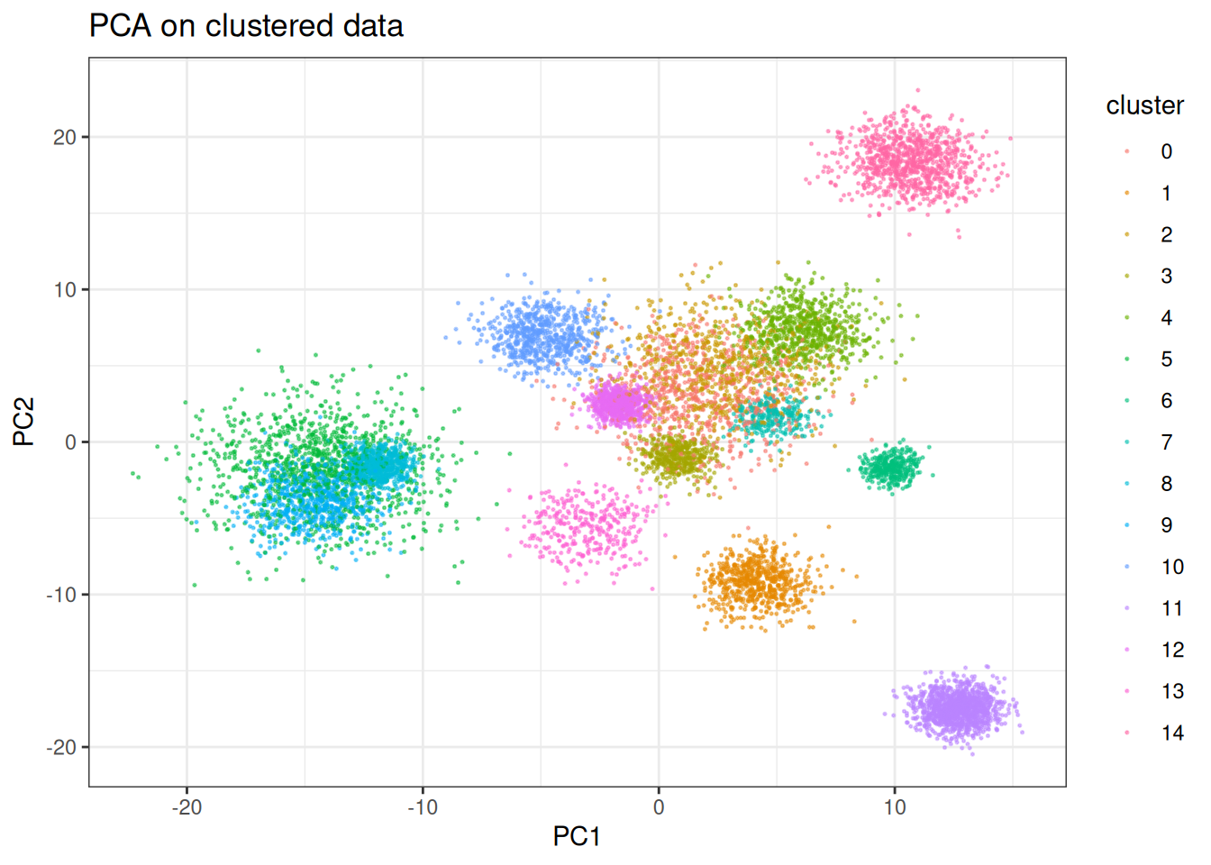
And now check PHATE:
phate_clusters <- phate(
  data = cluster_data$data,
  k = 15L,
  seed = 42L
)

phate_clusters_df <- as.data.table(phate_clusters) %>%
  `colnames<-`(c("PHATE1", "PHATE2")) %>%
  .[, cluster := as.factor(cluster_data$membership)]

ggplot(
  data = phate_clusters_df,
  mapping = aes(x = PHATE1, y = PHATE2)
) +
  geom_point(mapping = aes(colour = cluster), size = 0.75, alpha = 0.5) +
  theme_bw() +
  ggtitle("PHATE on clustered data")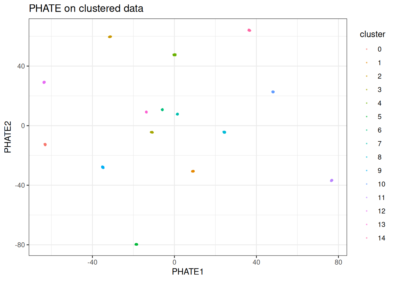
As expected, the clusters explode outward and are condensed into nearly single points. PHATE is trying to lay out a manifold that does not exist in this data. If your data looks like this, use t-SNE or UMAP instead.
Swiss role
The swiss role is a continuous manifold where PHATE should perform meaningfully better than t-SNE or UMAP. The diffusion process captures the smooth geometry of the roll rather than tearing it apart.
phate_swissrole <- phate(
  data = swissrole_data$data,
  k = 15L,
  knn_method = "exhaustive",
  seed = 42L
)

phate_swissrole_df <- as.data.table(phate_swissrole) %>%
  `colnames<-`(c("PHATE1", "PHATE2")) %>%
  .[, z_axis := swissrole_data$data[, 3]]

ggplot(
  data = phate_swissrole_df,
  mapping = aes(x = PHATE1, y = PHATE2)
) +
  geom_point(
    mapping = aes(fill = z_axis),
    shape = 21,
    size = 2,
    alpha = 0.5
  ) +
  scale_fill_viridis_c() +
  theme_bw() +
  ggtitle("PHATE on swissrole data")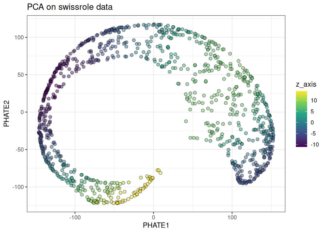
PHATE preserves the continuous colour gradient along the roll substantially better than t-SNE, and considerably better than UMAP. For manifolds like this, PHATE is the stronger choice.
Trajectory
The trajectory data is where PHATE was built to shine. Branching trajectories are the canonical use case.
phate_trajectory <- phate(
  data = trajectory_data$data,
  k = 15L,
  seed = 42L
)

phate_trajectory_df <- as.data.table(phate_trajectory) %>%
  `colnames<-`(c("PHATE1", "PHATE2")) %>%
  .[, branch := trajectory_data$membership]

ggplot(
  data = phate_trajectory_df[
    sample(1:nrow(phate_trajectory_df), nrow(phate_trajectory_df)),
  ],
  mapping = aes(x = PHATE1, y = PHATE2)
) +
  geom_point(
    mapping = aes(colour = branch),
    alpha = 0.5,
    size = 0.75
  ) +
  theme_bw() +
  scale_colour_viridis_c(option = "turbo") +
  ggtitle("PHATE on trajectory data")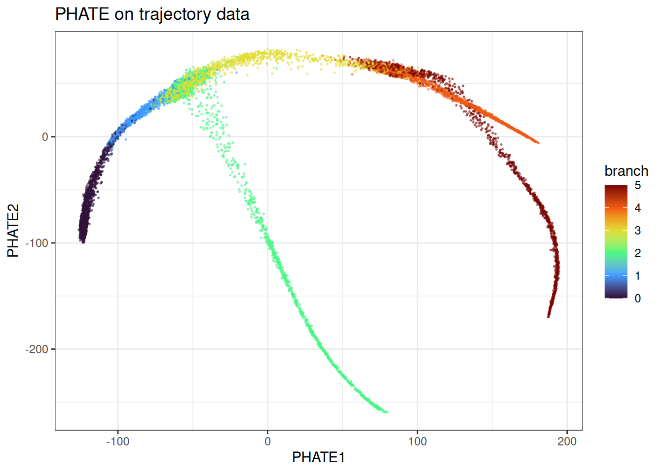
PHATE recovers the branching structure cleanly. The continuous progression along each branch is preserved, and the branch points are identifiable. This is the kind of data PHATE was designed for.
Using pre-computed kNN graphs
As with t-SNE, if you want to explore multiple parameter combinations without repeating the kNN search, you can precompute the graph and pass it directly.
precomputed_knn <- generate_knn_graph(
  data = trajectory_data$data,
  k = 15L,
  .verbose = FALSE
)

phate_from_knn <- phate(
  data = trajectory_data$data,
  knn = precomputed_knn,
  k = 15L,
  seed = 42L
)
#> Using provided kNN graph.

phate_from_knn_df <- as.data.table(phate_from_knn) %>%
  `colnames<-`(c("PHATE1", "PHATE2")) %>%
  .[, branch := trajectory_data$membership]

ggplot(
  data = phate_from_knn_df[
    sample(1:nrow(phate_from_knn_df), nrow(phate_from_knn_df)),
  ],
  mapping = aes(x = PHATE1, y = PHATE2)
) +
  geom_point(mapping = aes(colour = branch), alpha = 0.5, size = 0.75) +
  theme_bw() +
  scale_colour_viridis_c(option = "turbo") +
  ggtitle("PHATE from kNN graph (version 1)")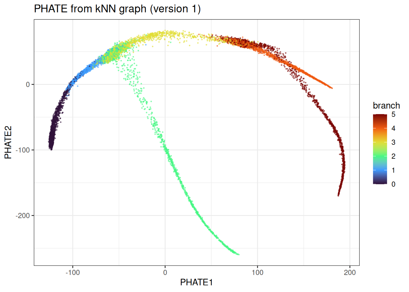
With the kNN graph fixed, we can quickly vary PHATE-specific parameters. For example, trying a fixed diffusion time rather than automatic selection:
phate_from_knn_fixed_t <- phate(
  data = trajectory_data$data,
  knn = precomputed_knn,
  k = 15L,
  phate_params = params_phate(t_custom = 10L),
  seed = 42L
)
#> Using provided kNN graph.

phate_from_knn_fixed_t_df <- as.data.table(phate_from_knn_fixed_t) %>%
  `colnames<-`(c("PHATE1", "PHATE2")) %>%
  .[, branch := trajectory_data$membership]

ggplot(
  data = phate_from_knn_fixed_t_df[
    sample(1:nrow(phate_from_knn_fixed_t_df), nrow(phate_from_knn_fixed_t_df)),
  ],
  mapping = aes(x = PHATE1, y = PHATE2)
) +
  geom_point(mapping = aes(colour = branch), alpha = 0.5, size = 0.75) +
  theme_bw() +
  scale_colour_viridis_c(option = "turbo") +
  ggtitle("PHATE from kNN graph (version 2)")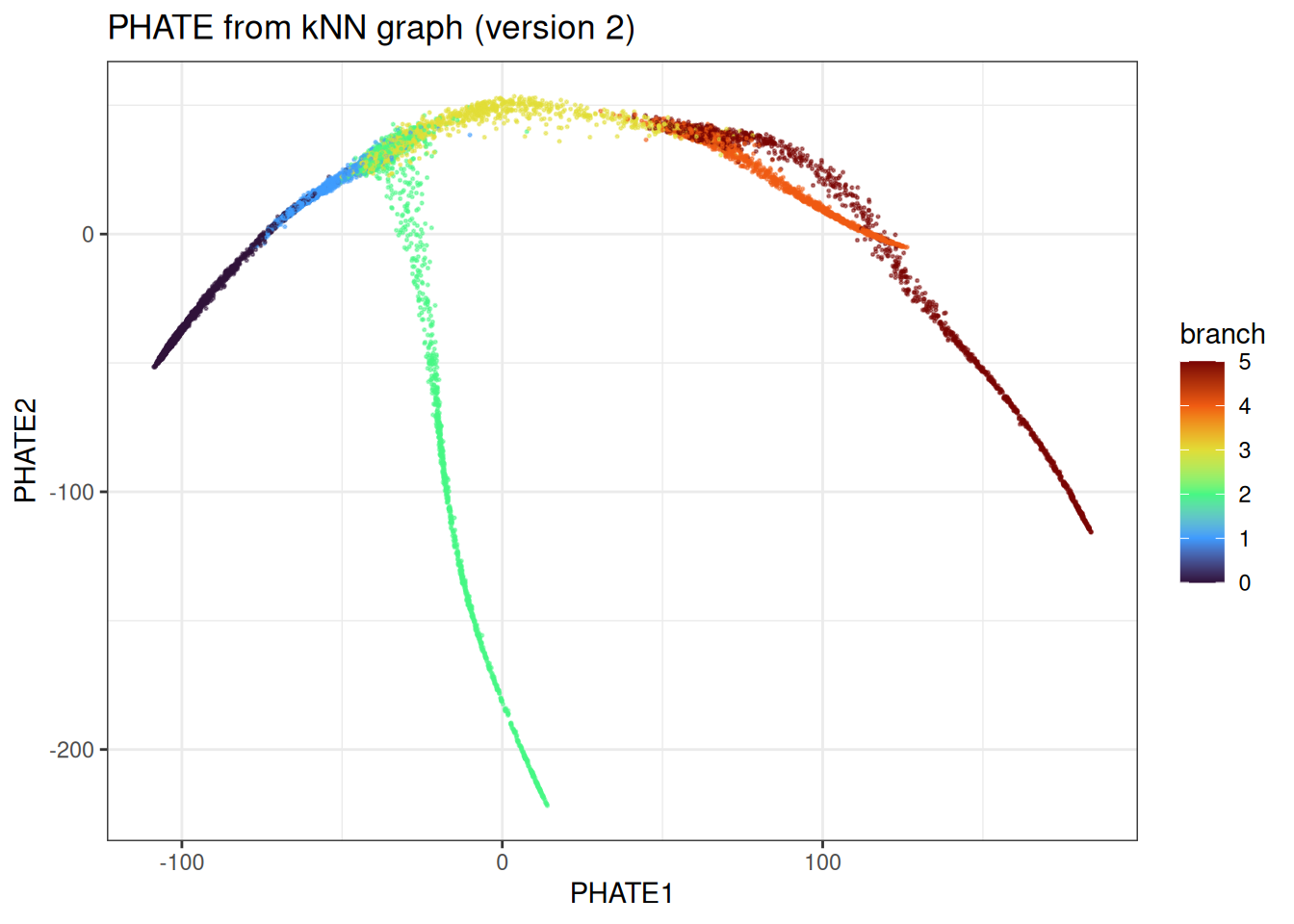
Landmark PHATE
For large datasets, computing and storing the full N x N diffusion operator is prohibitive — both in memory and computation. The landmark approach addresses this by selecting a small, representative subset of points (landmarks), running the full diffusion only over those, and then interpolating the remaining points into the landmark space. The default behaviour is to use 2048L in this package (if you wonder why 2048, it’s for the SIMD-acceleration in the k-means under the hood which work better on 2^x numbers).
The three landmark selection strategies available via landmark_method differ in how they choose these representative points:
-
"spectral"(default): landmarks are selected via spectral clustering on the affinity graph. This tends to give the most geometrically representative coverage, particularly for data with complex topology, but is the most expensive of the three. -
"random": landmarks are drawn uniformly at random. Fast, but coverage can be uneven in datasets with non-uniform density. -
"density": landmarks are drawn from a dampened node degree-weighted distribution. This makes it a bit more precise than pure random, but rare branches might be missed.
The number of landmarks is controlled by n_landmarks. As a rough guide, 500–2000 landmarks is sufficient for most datasets up to a few hundred thousand points. Too few and the interpolation will miss fine structure; too many and you lose most of the speed benefit. If you try running this on large data sets with n_landmarks = NULL, the function will warn you… It will be nasty on larger data sets as you have to materialise a N x N dense matrix, calculated the potential distances over N x N, instead of N x L, etc.
large_trajectory <- manifold_synthetic_data(
  type = "trajectory",
  n_samples = 50000L
)

phate_landmark <- phate(
  data = large_trajectory$data,
  k = 15L,
  phate_params = params_phate(
    n_landmarks = 1024L,
    landmark_method = "spectral"
  ),
  seed = 42L
)

phate_landmark_df <- as.data.table(phate_landmark) %>%
  `colnames<-`(c("PHATE1", "PHATE2")) %>%
  .[, branch := large_trajectory$membership]

ggplot(
  data = phate_landmark_df[
    sample(1:nrow(phate_landmark_df), nrow(phate_landmark_df)),
  ],
  mapping = aes(x = PHATE1, y = PHATE2)
) +
  geom_point(mapping = aes(colour = branch), alpha = 0.5, size = 0.75) +
  theme_bw() +
  scale_colour_viridis_c(option = "turbo") +
  ggtitle("PHATE with 1024 landmarks (spectral)")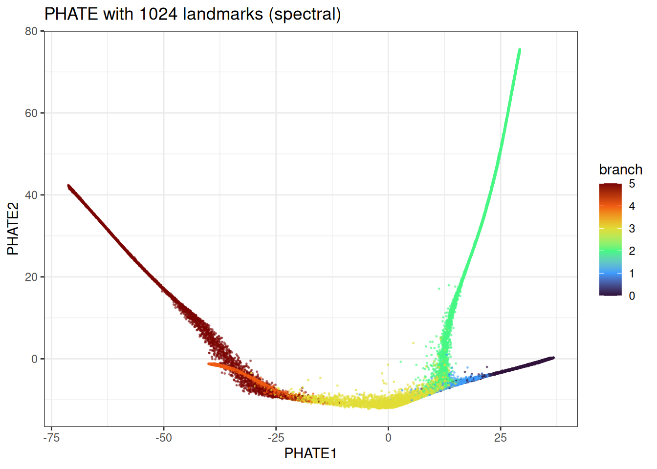
We can even further accelerate this with the density or random-based version
large_trajectory <- manifold_synthetic_data(
  type = "trajectory",
  n_samples = 50000L
)

phate_landmark <- phate(
  data = large_trajectory$data,
  k = 15L,
  phate_params = params_phate(
    n_landmarks = 1024L,
    landmark_method = "random"
  ),
  seed = 42L
)

phate_landmark_df <- as.data.table(phate_landmark) %>%
  `colnames<-`(c("PHATE1", "PHATE2")) %>%
  dplyr::mutate(branch = large_trajectory$membership)

ggplot(
  data = phate_landmark_df[
    sample(1:nrow(phate_landmark_df), nrow(phate_landmark_df)),
  ],
  mapping = aes(x = PHATE1, y = PHATE2)
) +
  geom_point(mapping = aes(colour = branch), alpha = 0.5, size = 0.75) +
  theme_bw() +
  scale_colour_viridis_c(option = "turbo") +
  ggtitle("PHATE with 1024 landmarks (random)")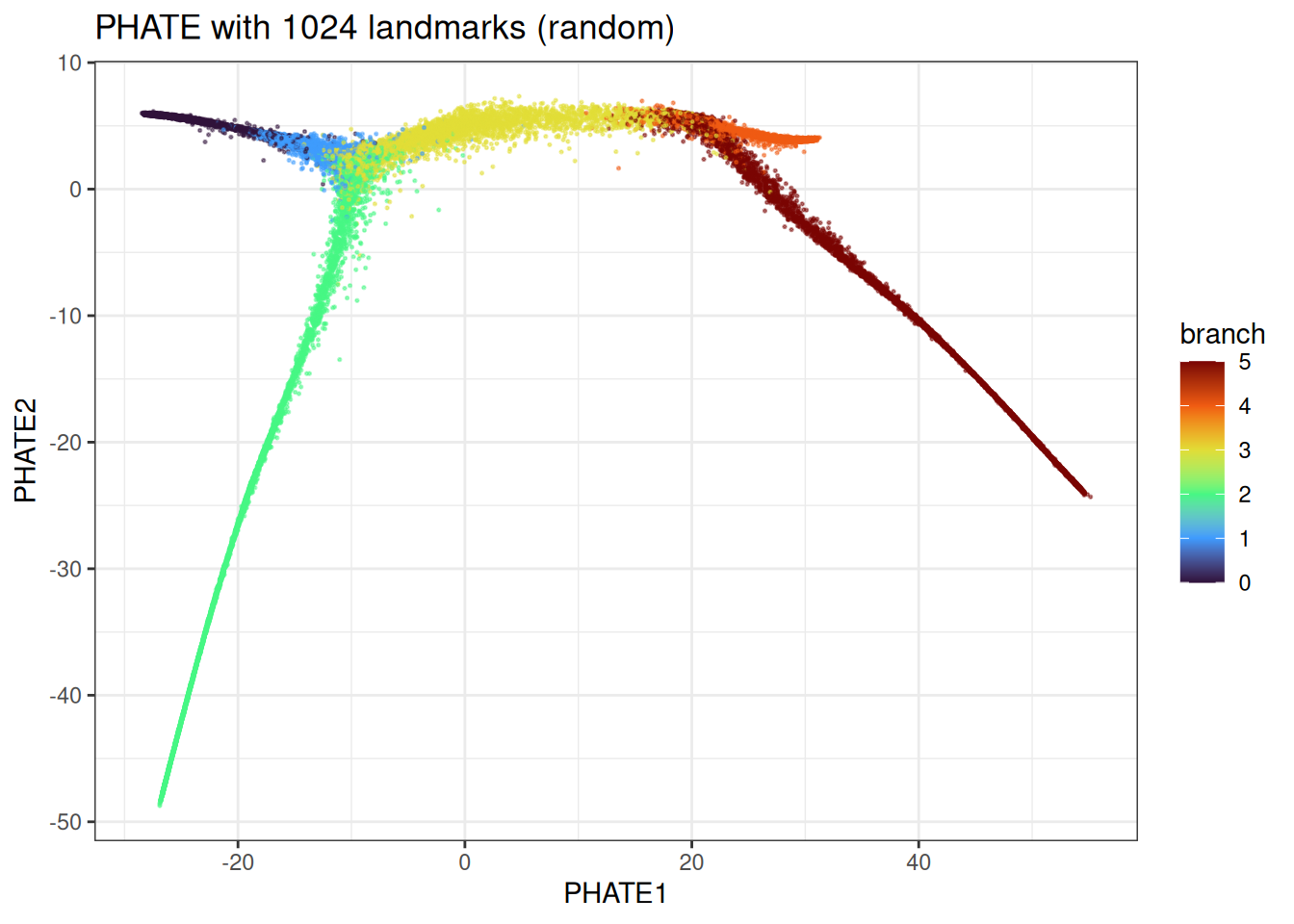
We can observe some differences here, but the overall trajectory is correctly identified.
Benchmarks
Let’s compare manifoldsR against phateR (the reference R implementation, itself a wrapper around the Python phate library) on the trajectory data.
local({
  env_name <- "r-manifolds"

  if (!reticulate::virtualenv_exists(env_name)) {
    reticulate::virtualenv_create(env_name)
    reticulate::virtualenv_install(
      env_name,
      packages = c("phate", "umap-learn", "numpy", "scipy")
    )
  }

  if (!reticulate::py_available()) {
    reticulate::use_virtualenv(env_name, required = TRUE)
  }

  missing_pkgs <- Filter(
    Negate(reticulate::py_module_available),
    c("phate", "umap")
  )
  if (length(missing_pkgs) > 0L) {
    reticulate::virtualenv_install(
      env_name,
      packages = c("phate", "umap-learn", "numpy", "scipy")
    )
  }
})
#> Using Python: /usr/bin/python3.12
#> Creating virtual environment 'r-manifolds' ...
#> + /usr/bin/python3.12 -m venv /home/runner/.virtualenvs/r-manifolds
#> Done!
#> Installing packages: pip, wheel, setuptools
#> + /home/runner/.virtualenvs/r-manifolds/bin/python -m pip install --upgrade pip wheel setuptools
#> Installing packages: numpy
#> + /home/runner/.virtualenvs/r-manifolds/bin/python -m pip install --upgrade --no-user numpy
#> Virtual environment 'r-manifolds' successfully created.
#> Using virtual environment 'r-manifolds' ...
#> + /home/runner/.virtualenvs/r-manifolds/bin/python -m pip install --upgrade --no-user phate umap-learn numpy scipy

benchmark_data <- manifold_synthetic_data(
  type = "trajectory",
  n_samples = 10000L
)

microbenchmark::microbenchmark(
  phateR = {
    phateR::phate(
      data = benchmark_data$data,
      knn = 5L,
      n.jobs = -1,
      verbose = FALSE
    )
  },
  manifold_phate = {
    phate(
      data = benchmark_data$data,
      k = 5L,
      seed = 42L,
      .verbose = FALSE
    )
  },
  times = 1L
)
#> Unit: seconds
#>            expr       min        lq      mean    median        uq       max
#>          phateR 11.538472 11.538472 11.538472 11.538472 11.538472 11.538472
#>  manifold_phate  9.406992  9.406992  9.406992  9.406992  9.406992  9.406992
#>  neval
#>      1
#>      1
And on a larger data set with additionally the random landmark version
benchmark_data_large <- manifold_synthetic_data(
  type = "trajectory",
  n_samples = 100000L
)

microbenchmark::microbenchmark(
  phateR = {
    phateR::phate(
      data = benchmark_data_large$data,
      knn = 5L,
      npca = 100L,
      n.jobs = -1,
      verbose = FALSE
    )
  },
  manifold_phate_spectral = {
    phate(
      data = benchmark_data_large$data,
      k = 5L,
      knn_method = "nndescent", # good allrounder for larger data sets
      seed = 42L,
      .verbose = FALSE
    )
  },
  manifold_phate_random = {
    phate(
      data = benchmark_data_large$data,
      k = 5L,
      knn_method = "nndescent", # good allrounder for larger data sets
      phate_params = params_phate(landmark_method = "random"),
      seed = 42L,
      .verbose = FALSE
    )
  },
  times = 1L
)
#>     SGD-MDS may not have converged: stress changed by -1.9% in final iterations. Consider increasing n_iter or adjusting learning_rate.
#> Unit: seconds
#>                     expr      min       lq     mean   median       uq      max
#>                   phateR 55.77747 55.77747 55.77747 55.77747 55.77747 55.77747
#>  manifold_phate_spectral 61.70343 61.70343 61.70343 61.70343 61.70343 61.70343
#>    manifold_phate_random 15.65289 15.65289 15.65289 15.65289 15.65289 15.65289
#>  neval
#>      1
#>      1
#>      1
As with t-SNE and UMAP, the speed advantage of the Rust implementation comes from the entire pipeline — kNN construction, kernel computation, diffusion, and MDS — running within the Rust kernel without round-tripping through Python in this case. Usually, the differences become more pronounced with larger data sets.