library(manifoldsR)
library(magrittr)
library(ggplot2)
library(data.table)
#>
#> Attaching package: 'data.table'
#> The following object is masked from 'package:base':
#>
#>     %notin%
Using ForceAtlas2
2026-09-25
ForceAtlas2 in manifoldsR
manifoldsR ships a Rust implementation of ForceAtlas2 (FA2), the force directed layout from Gephi. Single cell folks know it from scanpy’s draw_graph and from PAGA initialised layouts.
Intro
FA2 treats the kNN graph as a physical system. Every node pushes every other node away with a force of 1/d, scaled by the node masses (1 + degree, so hubs push harder). Every edge pulls its two ends together, linearly with distance, or logarithmically with lin_log = TRUE. Gravity pulls everything towards the origin so disconnected components don’t drift off. Step sizes follow Gephi’s adaptive speed: nodes that swing back and forth slow down, nodes that move steadily speed up. The all-pairs repulsion runs on a Barnes-Hut tree.
How is that different from UMAP? UMAP samples edges and negative pairs stochastically and optimises a cross-entropy loss. FA2 visits every edge every epoch and has no loss at all, just forces. There’s also no min_dist or spread: the scale of the layout comes out of the balance between scaling_ratio (repulsion) and the edge weights (attraction).
There are two entry points:
-
forceatlas2()takes the data (or aNearestNeighboursobject), builds the UMAP fuzzy union graph like scanpy does and lays it out. -
forceatlas2_from_graph()takes any undirectedigraphobject, e.g. an SNN graph, a graph from another package or one you built by hand.
FA2 needs a symmetric graph, since each edge pulls both of its ends equally. The first entry point guarantees that by construction. For the second, an undirected igraph object is symmetric by definition, so directed graphs are rejected.
Running ForceAtlas2
We use the same synthetic data as in the UMAP vignette.
cluster_data <- manifold_synthetic_data(
  type = "cluster",
  n_samples = 25000L
)

trajectory_data <- manifold_synthetic_data(
  type = "trajectory",
  n_samples = 25000L
)
Clustered data
fa2_clusters <- forceatlas2(
  data = cluster_data$data,
  k = 15L
)

fa2_clusters_df <- as.data.table(fa2_clusters) %>%
  `colnames<-`(c("FA1", "FA2")) %>%
  .[, cluster := as.factor(cluster_data$membership)]

ggplot(
  data = fa2_clusters_df,
  mapping = aes(x = FA1, y = FA2)
) +
  geom_point(mapping = aes(colour = cluster), size = 0.75, alpha = 0.5) +
  theme_bw() +
  ggtitle("ForceAtlas2 on clustered data")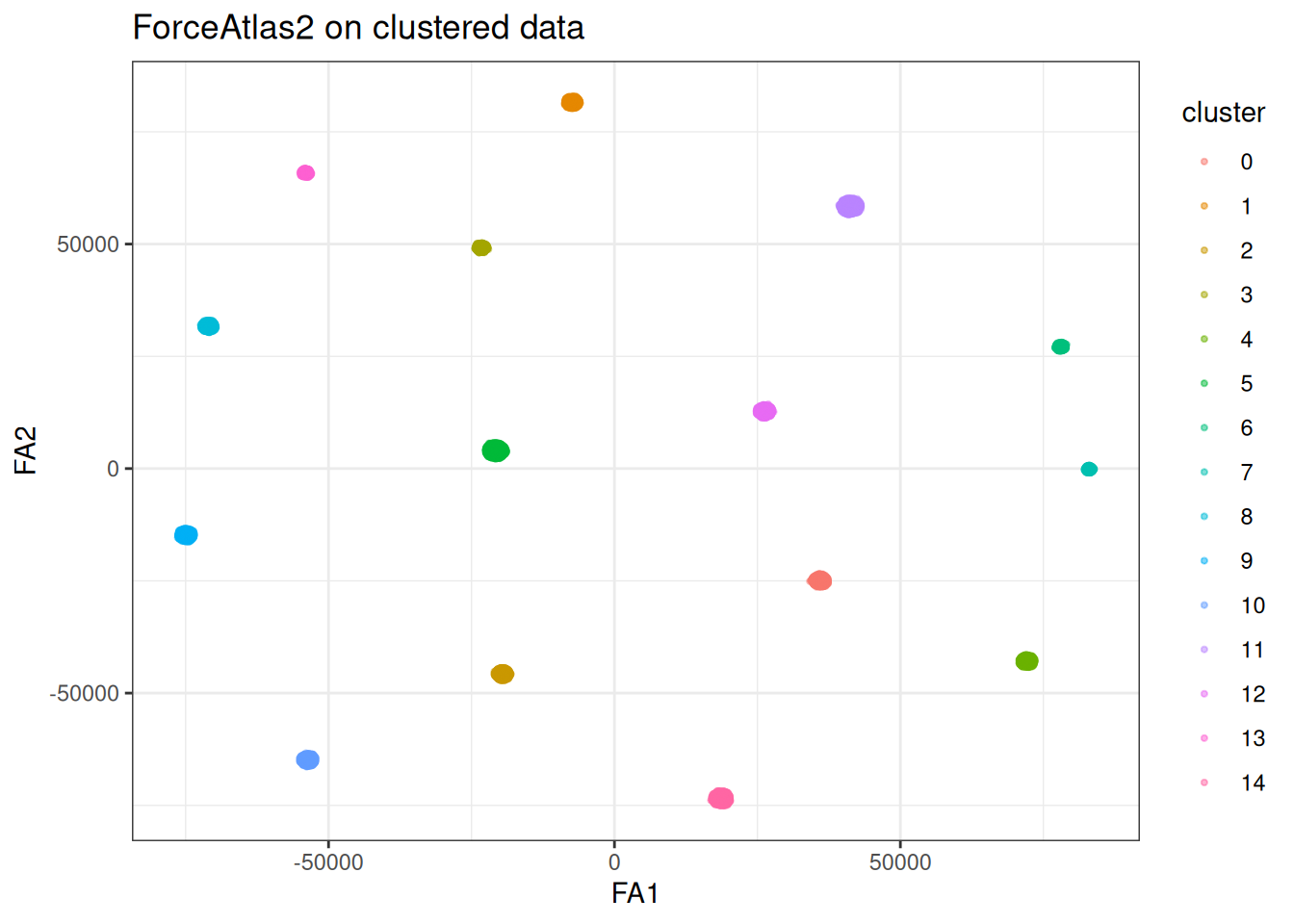
And UMAP on the same data for comparison:
umap_clusters <- umap(
  data = cluster_data$data,
  k = 15L
)
#> Using n_epochs = 500 (dataset <10k samples or adam_parallel optimiser)

umap_clusters_df <- as.data.table(umap_clusters) %>%
  `colnames<-`(c("UMAP1", "UMAP2")) %>%
  .[, cluster := as.factor(cluster_data$membership)]

ggplot(
  data = umap_clusters_df,
  mapping = aes(x = UMAP1, y = UMAP2)
) +
  geom_point(mapping = aes(colour = cluster), size = 0.75, alpha = 0.5) +
  theme_bw() +
  ggtitle("UMAP on clustered data")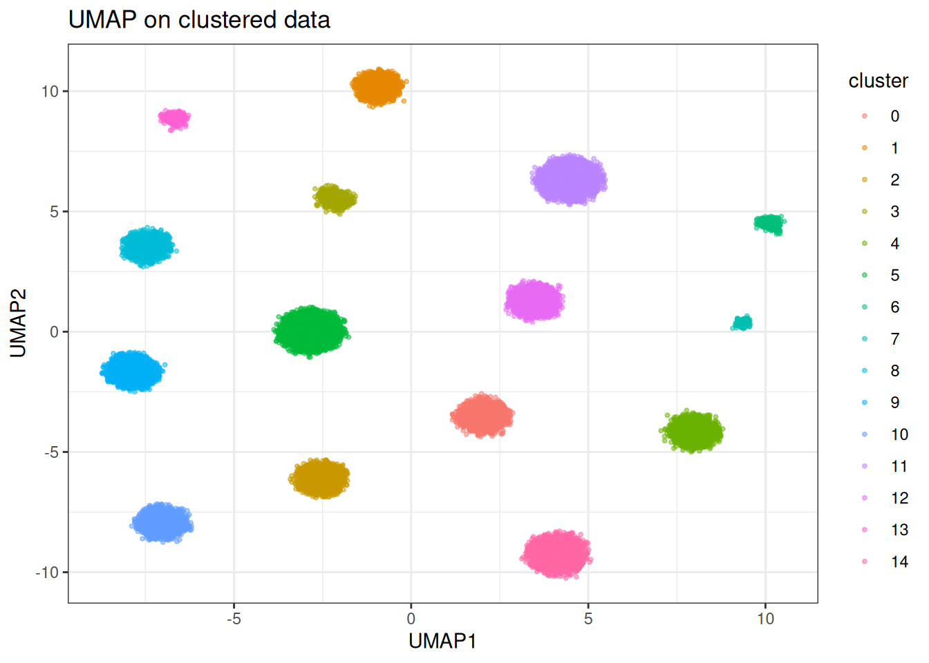
Both separate all 15 clusters, and the global arrangement is near identical, since both start from the same spectral initialisation. The difference is inside the clusters: with linear attraction and a dense within-cluster graph, FA2 pulls each cluster into a tight blob. Also note the axes. FA2 coordinates live on Gephi’s scale, so tens of thousands are normal. Only the relative positions carry meaning.
Trajectory
Trajectories are where force directed layouts get used most in single cell work. Let’s see how FA2 handles the branching data.
fa2_trajectory <- forceatlas2(
  data = trajectory_data$data,
  k = 15L
)

fa2_trajectory_df <- as.data.table(fa2_trajectory) %>%
  `colnames<-`(c("FA1", "FA2")) %>%
  .[, branch := trajectory_data$membership]

# shuffle the rows to not over-plot the later branches
ggplot(
  data = fa2_trajectory_df[sample(.N)],
  mapping = aes(x = FA1, y = FA2)
) +
  geom_point(mapping = aes(colour = branch), size = 0.75, alpha = 0.5) +
  theme_bw() +
  ggtitle("ForceAtlas2 on trajectory data")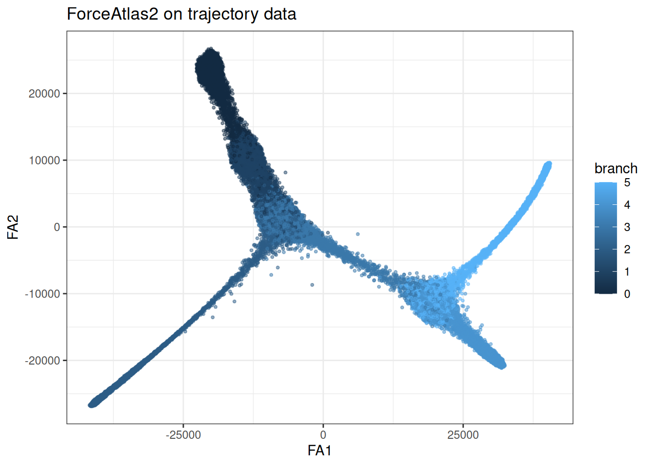
The branching structure survives: every branch stays attached to its parent and the whole thing reads as one connected tree rather than a set of islands.
The knobs
All knobs live in params_fa2(). The ones that matter:
-
scaling_ratio: repulsion strength. Bigger values spread everything out. -
gravity: pull towards the origin. Crank it up if small components float away, lower it if everything gets squashed into a ball. -
lin_log: logarithmic attraction. Gives tighter communities. -
dissuade_hubs: divides the attraction by the node mass, so hubs get pushed to the edge of their community. -
n_epochs: FA2 has no learning rate schedule to anneal, so more epochs mean a more settled layout. The default is500.
theta controls the Barnes-Hut approximation (0 gives the exact repulsion) and jitter_tolerance how much swinging the adaptive speed tolerates. Leave them alone unless you know why you’re touching them.
Here’s LinLog mode on the clustered data:
fa2_linlog <- forceatlas2(
  data = cluster_data$data,
  k = 15L,
  fa2_params = params_fa2(lin_log = TRUE)
)

fa2_linlog_df <- as.data.table(fa2_linlog) %>%
  `colnames<-`(c("FA1", "FA2")) %>%
  .[, cluster := as.factor(cluster_data$membership)]

ggplot(
  data = fa2_linlog_df,
  mapping = aes(x = FA1, y = FA2)
) +
  geom_point(mapping = aes(colour = cluster), size = 0.75, alpha = 0.5) +
  theme_bw() +
  ggtitle("ForceAtlas2 (LinLog) on clustered data")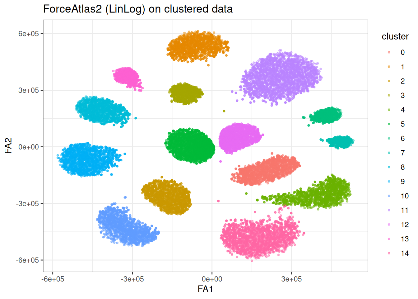
Same arrangement as before, but the clusters open up and you can see their internal spread again. The logarithmic attraction grows much slower with distance, so the within-cluster pull no longer crushes everything into a point.
Bring your own graph
Already have a graph? Hand it to forceatlas2_from_graph(). Here we build a plain unweighted kNN graph in igraph from a NearestNeighbours object. igraph::simplify() merges the mutual neighbours (A in B’s list and B in A’s) into one edge and drops self-loops.
knn <- generate_knn_graph(
  data = trajectory_data$data,
  k = 15L
)

knn_idx <- get_idx_mat(knn)

knn_graph <- igraph::graph_from_edgelist(
  cbind(rep(seq_len(nrow(knn_idx)), ncol(knn_idx)), as.vector(knn_idx)),
  directed = FALSE
) %>%
  igraph::simplify()

knn_graph
#> IGRAPH 8204ad0 U--- 25000 323921 --
#> + edges from 8204ad0:
#>  [1] 1-- 114 1-- 133 1-- 309 1-- 528 1-- 643 1--1003 1--1081 1--1100 1--1213
#> [10] 1--1219 1--1274 1--1477 1--1478 1--1577 1--2246 1--2260 1--2495 1--2541
#> [19] 1--2601 1--2784 1--3249 1--3279 1--3843 1--4052 1--4080 2--  82 2-- 118
#> [28] 2-- 123 2-- 200 2-- 208 2-- 253 2-- 322 2-- 379 2-- 423 2-- 566 2-- 623
#> [37] 2-- 742 2-- 887 2-- 983 2--1120 2--1155 2--1199 2--1377 2--1380 2--1420
#> [46] 2--1491 2--1526 2--1649 2--2213 2--2338 2--2364 2--2412 2--2468 2--2784
#> [55] 2--2798 2--2854 2--2860 2--2874 2--2968 2--3214 2--3234 2--3252 2--3324
#> [64] 2--3472 2--3479 2--3627 2--3684 2--3713 2--3780 2--3810 2--3892 2--3936
#> [73] 2--4056 2--4080 2--4105 2--4125 3--  26 3-- 819 3--1221 3--2017 3--2317
#> + ... omitted several edges
If the graph has a weight edge attribute, FA2 uses it (raised to the power edge_weight_influence). This one doesn’t, so every edge weighs 1. Without init, the layout starts from random positions:
fa2_graph <- forceatlas2_from_graph(graph = knn_graph)

fa2_graph_df <- as.data.table(fa2_graph) %>%
  `colnames<-`(c("FA1", "FA2")) %>%
  .[, branch := trajectory_data$membership]

ggplot(
  data = fa2_graph_df[sample(.N)],
  mapping = aes(x = FA1, y = FA2)
) +
  geom_point(mapping = aes(colour = branch), size = 0.75, alpha = 0.5) +
  theme_bw() +
  ggtitle("ForceAtlas2 on an unweighted kNN graph (random init)")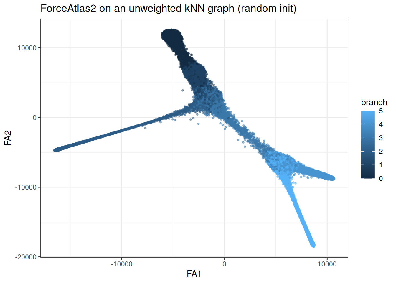
You can also start from an existing layout. Any n x 2 matrix works; here we use a UMAP of the same data, reusing the kNN search:
umap_init <- umap(
  data = trajectory_data$data,
  knn = knn,
  k = 15L
)
#> Using n_epochs = 500 (dataset <10k samples or adam_parallel optimiser)
#> Using provided kNN graph.

fa2_graph_warm <- forceatlas2_from_graph(
  graph = knn_graph,
  init = umap_init
)

fa2_graph_warm_df <- as.data.table(fa2_graph_warm) %>%
  `colnames<-`(c("FA1", "FA2")) %>%
  .[, branch := trajectory_data$membership]

ggplot(
  data = fa2_graph_warm_df[sample(.N)],
  mapping = aes(x = FA1, y = FA2)
) +
  geom_point(mapping = aes(colour = branch), size = 0.75, alpha = 0.5) +
  theme_bw() +
  ggtitle("ForceAtlas2 on an unweighted kNN graph (UMAP init)")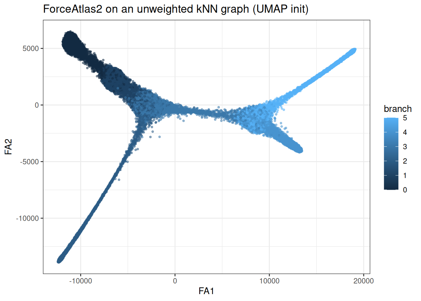
Both starts end in the same tree, just rotated and mirrored. The unweighted kNN graph carries enough structure on its own here; the init mostly decides the orientation.
Only the optimisation parameters in params_fa2() apply here. The graph building and initialisation ones (local_connectivity, bandwidth, init, randomised) belong to forceatlas2().