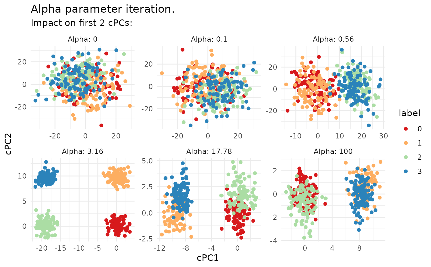
Plot various alphas for the contrastive PCA

This function will plot various alphas to highlight the most interesting alpha parameters akin to the implementation of contrastive PCA in Python.

Usage

c_pca_plot_alphas(
  object,
  label_column = NULL,
  min_alpha = 0.1,
  max_alpha = 100,
  n_alphas = 10L,
  .verbose = TRUE
)

Arguments

object

The underlying class, see BulkCoExp(). You need to apply contrastive_pca_processing() to the function for this method to work. Checkmate will raise errors otherwise.

label_column

An optional sample label column. Needs to exist in the meta_data of the BulkCoExp class.

min_alpha

Minimum alpha to test.

max_alpha

Maximum alpha to test.

n_alphas

Number of alphas to test. The function will generate a series of alphas from log(min_alpha) to log(max_alpha) to test out.

.verbose

Controls verbosity of function.

Value

A ggplot showing the impact of various alpha parameters on the samples in form of 2D plots.

References

Abid, et al., Nature Communications, 2018

Examples

# how the group separation responds to alpha
cpca_data <- synthetic_c_pca_data()
target <- t(cpca_data$target)
background <- t(cpca_data$background)
meta <- data.table::data.table(
  sample_id = rownames(target),
  grp = cpca_data$target_labels
)
obj <- BulkCoExp(target, meta)
obj <- preprocess_bulk_coexp(obj, .verbose = FALSE)
obj <- contrastive_pca_processing(obj, background, .verbose = FALSE)
c_pca_plot_alphas(obj, label_column = "grp", n_alphas = 6L, .verbose = FALSE)