Contrastive PCA

bixverse provides an implementation of the contrastive PCA algorithm from Abid, et al.. This vignette will show you how to run the algorithm with some synthetic data.

library(bixverse)
library(data.table)

Intro

Standard PCA finds the directions of maximum variance in your data. This is often exactly what you want — but not always. In many biological settings, the dominant sources of variance are technical or contextual: batch effects, cell cycle, sequencing depth, or broad signals shared across all conditions. These swamp the more subtle biological variation you actually care about.

Contrastive PCA addresses this directly. Instead of decomposing the covariance of your target data alone, it works with the contrastive covariance matrix:

$C_\alpha = \Sigma_{target} - \alpha \cdot \Sigma_{background}$

where $\Sigma_{target}$ and $\Sigma_{background}$ are the covariance matrices of your target and background datasets, respectively. The eigenvectors of $C_\alpha$ define the contrastive principal components — directions that capture variance enriched in the target relative to the background. The parameter $\alpha \geq 0$ controls how aggressively the background signal is subtracted.

At $\alpha = 0$ , contrastive PCA reduces to standard PCA on the target data. As $\alpha$ increases, directions shared with the background are progressively suppressed, and the components increasingly reflect structure unique to the target. At very high $\alpha$ , you risk over-subtracting: genuine signal that happens to be partially present in the background gets removed as well.

Choosing $\alpha$ is therefore the central modelling decision. There is no universally correct value — it depends on how much background signal you want to remove and how much target-specific signal remains. The typical workflow is to scan a range of $\alpha$ values and select one that produces meaningful separation in your target groups, which bixverse makes straightforward.

One important caveat: contrastive PCA assumes your background dataset is a reasonable proxy for the unwanted variance. A poorly chosen background — one that shares little covariance with the dominant noise in your target — will produce components that are just standard PCs in disguise. Conversely, a background that is too similar to your target will over-subtract and destroy biological signal. The method works best when you have a principled choice of background, such as healthy controls alongside diseased samples, or an unlabelled reference population in a single-cell context.

Data

Let’s explore first the synthetic data (same as from the original authors).

cpca_test_data <- synthetic_c_pca_data()

plot(cpca_test_data)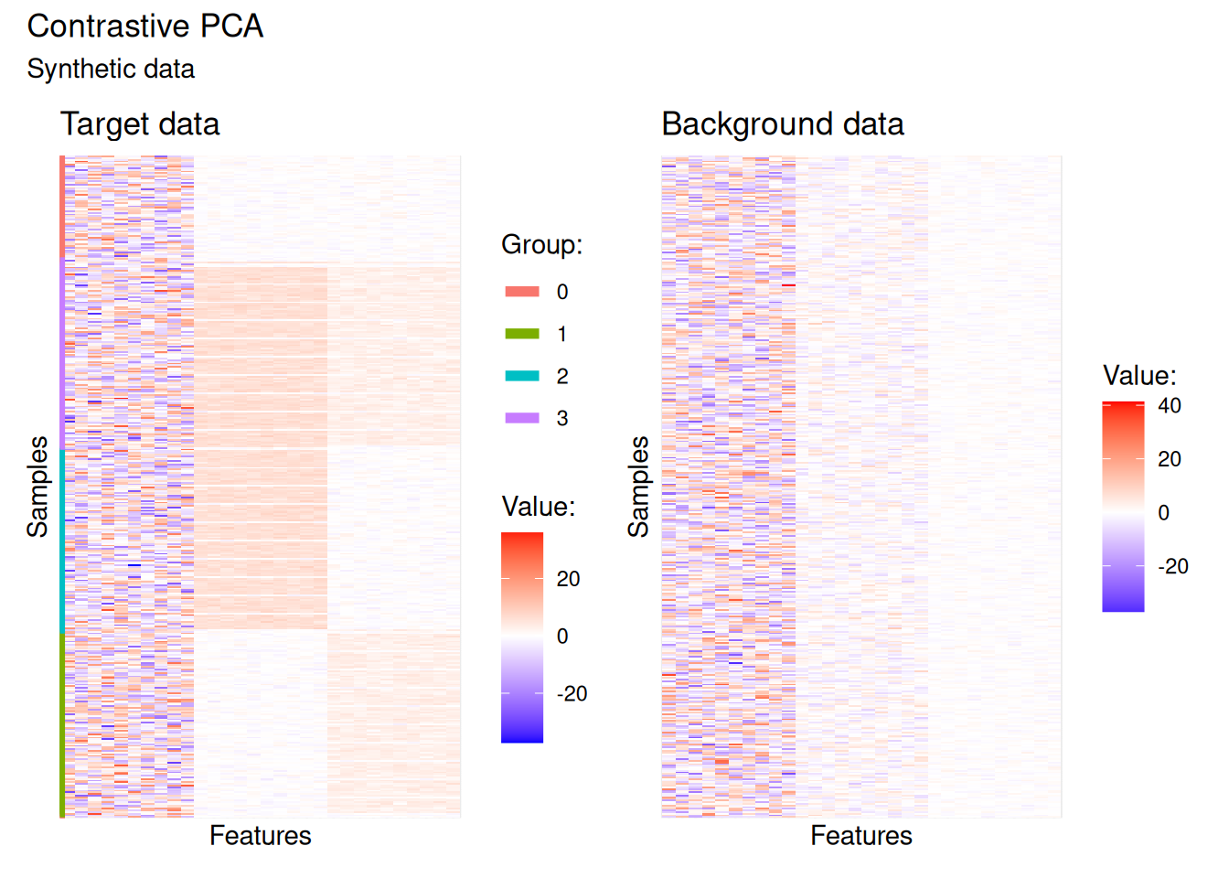

Synthetic data visualisation for contrastive PCA analysis

The pre-dominant signal sits in the first third of features — essentially noise — which makes it quite difficult to distinguish the four groups in the target data. The background data reproduces the same dominant signal but lacks the more subtle structure. This makes it an ideal candidate for contrastive PCA: the background encodes what we want to remove, and the target contains what we want to recover.

Explore the alpha parameter space

Let’s prepare the data for downstream analysis. Contrastive PCA in bixverse operates on a BulkCoExp object — the same class used for co-expression module analysis — built on S7.

raw_data <- t(cpca_test_data$target)
background_mat <- t(cpca_test_data$background)

sample_meta <- data.table(
  sample_id = rownames(raw_data),
  grp = cpca_test_data$target_labels
)

cpca_obj <- BulkCoExp(
  raw_data = raw_data,
  meta_data = sample_meta
)

# This function allows you to do scaling, HVG selection, etc.
# We won't be doing any of that here.
cpca_obj <- preprocess_bulk_coexp(cpca_obj)
#> A total of 30 genes will be included.

Next we supply the background data, which triggers computation of both covariance matrices internally.

cpca_obj <- contrastive_pca_processing(
  cpca_obj,
  background_mat = background_mat
)
#> A total of 30 features/genes were identified

The object is now ready to explore the alpha parameter space. bixverse provides a convenience function that runs contrastive PCA across a grid of $\alpha$ values and plots the resulting two-dimensional embeddings, coloured by a metadata column of your choice. This gives you an immediate visual sense of where meaningful separation emerges.

c_pca_plot_alphas(
  cpca_obj,
  label_column = "grp",
  n_alphas = 10L,
  max_alpha = 100
)
#> Found the grp in the meta data. Adding labels to the graph.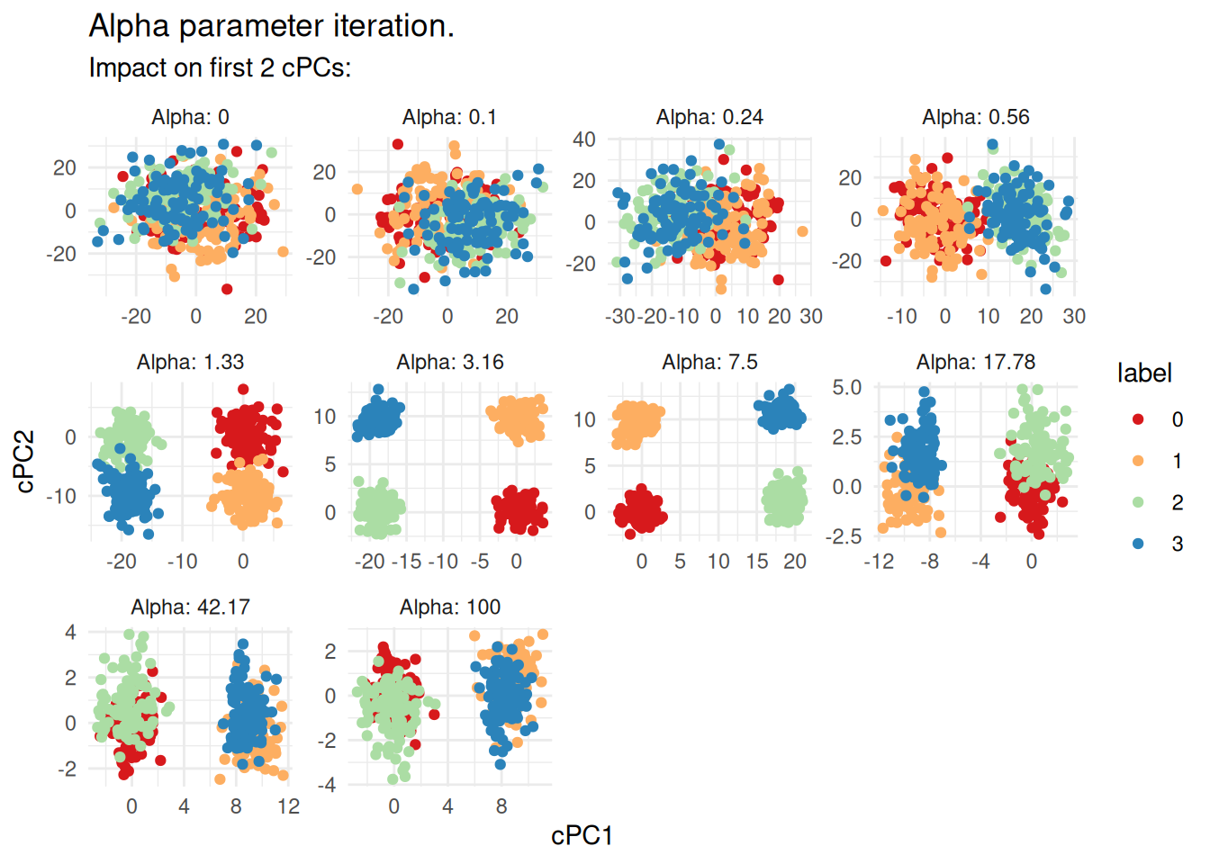

Impact of the alpha parameter on the ability to distinguish the groups

At $\alpha = 0$ the embedding is essentially standard PCA — dominated by the shared noise — and the four groups are indistinguishable. In the range of roughly $\alpha \approx 1.5$ to $10$ , the groups become clearly separated as the background signal is progressively removed. At higher values the embedding starts to degrade, consistent with over-subtraction. For this dataset, something in the range $\alpha \in [2, 5]$ looks reasonable.

Run contrastive PCA and extract the results

Once you have settled on an $\alpha$ , running the full decomposition and extracting the factors and loadings is straightforward:

cpca_obj <- contrastive_pca(
  cpca_obj,
  alpha = 2.5,
  no_pcs = 10L
)

# Extract the loadings (features x components)
c_pca_loadings <- get_c_pca_loadings(cpca_obj)

# Extract the factors (samples x components)
c_pca_factors <- get_c_pca_factors(cpca_obj)

The loadings describe which features contribute to each contrastive component and can be used for downstream gene set enrichment or feature interpretation. The factors are the low-dimensional sample coordinates and can feed directly into clustering, visualisation (e.g., UMAP), or differential analysis.

For further ideas on what to do with the output, see Abid, et al..