library(bixverse)
library(magrittr)
library(data.table)Genetic diffusion and community detections
Genetic diffusion and community detections
This vignette shows how to leverage networks to “diffuse” genetic information (to note, this could be any other type of seeding information) over these to create ranks of genes based on “diffusion heat”, calculate the predictive power of these genes against some gold standard genes, and also generate communities within the networks of “genetically privileged” mechanisms. The functions in the package have been inspired by work from Fang et al., Paull et al., Barrio-Hernandez et al., and Rosenthal et al..
Data
To exemplify the functions here, we will be using synthetic data, but you can easily adopt the workflow with any sets of seed genes and networks. We will create a barabasi graph of 100 nodes as an undirected network. Most biological networks follow a scale-free topology. For the seed genes, we will be sampling two sets based on the node degree distribution.
set.seed(123)

no_nodes <- 100L

barabasi_graph <- igraph::sample_pa(no_nodes, directed = FALSE)

node_names <- sprintf("genes%i", 1:no_nodes)

igraph::V(barabasi_graph)$name <- node_names

# The classes expects a data.table representing the edges
# Weighted and directed graphs are supported
edge_data <- setDT(igraph::as_data_frame(barabasi_graph))

# We will be creating two diffusion vectors based on the degree distribution
# and one set of gold standard genes
probs <- igraph::degree(barabasi_graph) / sum(igraph::degree(barabasi_graph))

genes_1 <- sample(
  igraph::V(barabasi_graph)$name,
  size = 5,
  prob = probs
)
genes_2 <- sample(
  igraph::V(barabasi_graph)$name,
  size = 8,
  prob = probs
)

diffusion_vector_1 <- rep(1, length(genes_1)) %>% `names<-`(genes_1)
diffusion_vector_2 <- rep(1, length(genes_2)) %>% `names<-`(genes_2)
gold_standard_genes <- sample(
  igraph::V(barabasi_graph)$name,
  size = 6,
  prob = probs
)
Running a single diffusion
To generate the class, you run
diffusion_obj <- NetworkDiffusions(
  edge_data,
  weighted = FALSE,
  directed = FALSE
)
For just running a single diffusion from a single set, you can do:
diffusion_obj <- diffuse_seed_nodes(
  object = diffusion_obj,
  diffusion_vector = diffusion_vector_1,
  summarisation = "max"
)

# Should you have duplicated names in the diffusion vector, the function
# provides different summarisation methods for the underlying scores
bixverse offers a permutation-based test, using degree matched samplings to calculate Z-scores for each node. This is based on Rust-accelerated, parallelised permutations.
diffusion_obj <- permute_seed_nodes(
  object = diffusion_obj,
  perm_iters = 1000L,
  .verbose = FALSE
)
You can access the data via S7 properties
diffusion_res <- get_diffusion_vector(diffusion_obj)
permutation_res <- get_diffusion_perms(diffusion_obj)

par(mfrow = c(1, 2))

hist(diffusion_res, xlab = "PPR score", main = "Diffusion result")
hist(permutation_res, xlab = "Z score", main = "Permutation result")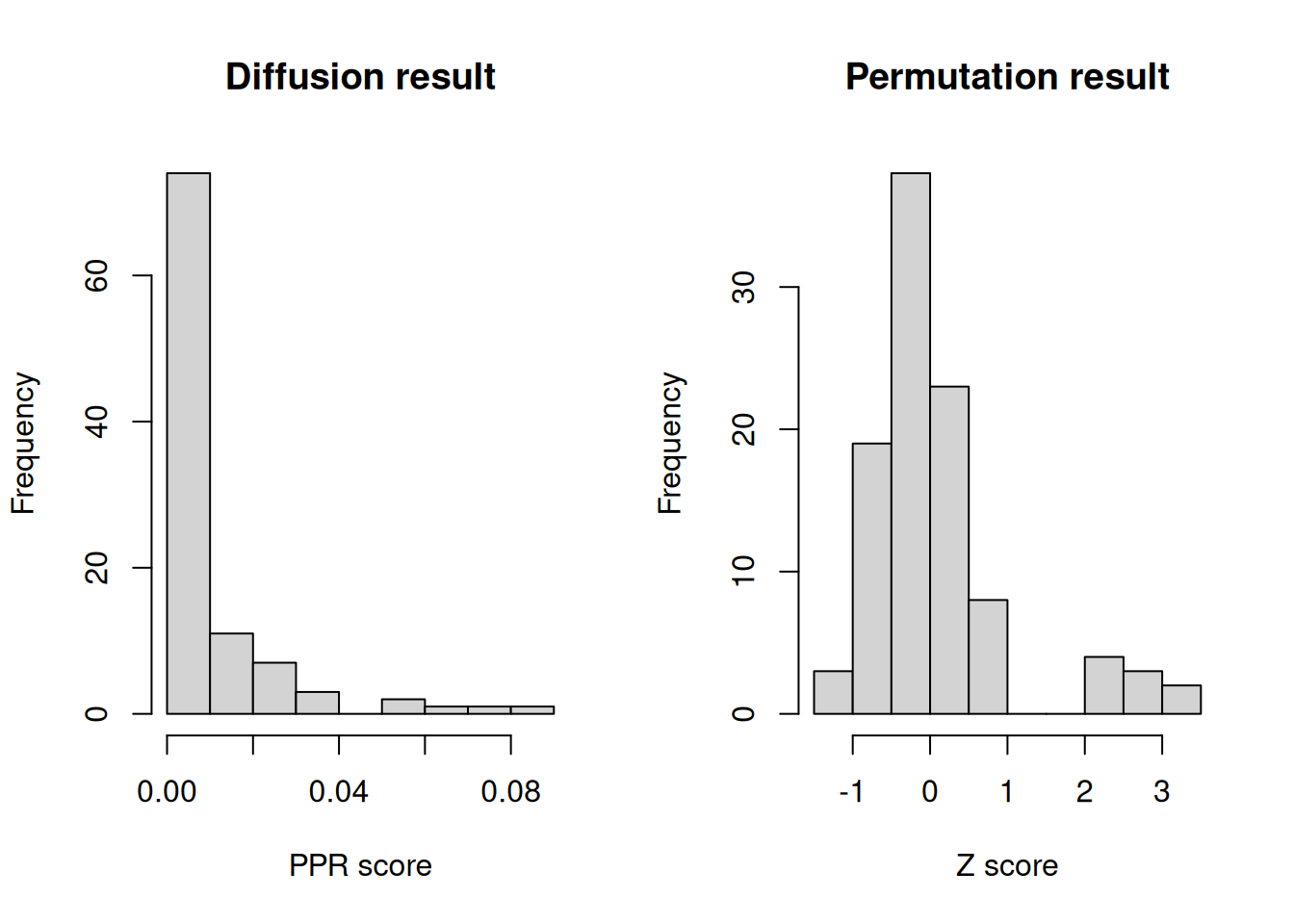
We can appreciated that there is a tail of values receiving more “diffuion heat” than expected just by topology properties of the network.
Assessing the recovery of gold standard genes
To assess if the diffusions are useful to start with, you can run:
auc_results <- calculate_diffusion_auc(
  object = diffusion_obj,
  hit_nodes = gold_standard_genes,
  permutation_test = TRUE # This will do permutation and generate Z-scores
)

print(
  sprintf(
    "The AUC of the diffuion is %.3f.",
    auc_results$auc
  )
)
#> [1] "The AUC of the diffuion is 0.589."
print(
  sprintf(
    "The Z-score based on random permutations is %.3f.",
    auc_results$z
  )
)
#> [1] "The Z-score based on random permutations is 0.764."
As this is random data, we observe an AUC of just 0.589 and a corresponding Z-score of 0.764, indicating that the diffusion is not very informative compared to random sets of gold standard genes.
Generation of communities with high diffusion heat
We provide function to identify regions in the graph that have higher diffusion heat (for e.g., ‘genetically privileged’ communities akin to Barrio-Hernandez et al.). We provide two options to return the initial network:
- Proportion of highest scoring nodes in the network (as in the intial paper).
- p-value based, i.e., you need to have run the permutations.
Verion 1 is run here:
diffusion_obj <- community_detection(
  object = diffusion_obj,
  community_params = params_community_detection(
    min_nodes = 5L,
    threshold_type = "prop_based",
    min_seed_nodes = 1L
  )
)

results_v1 <- get_results(diffusion_obj)
head(results_v1)
#>    cluster_id node_id      ks_pval cluster_size seed_nodes_no diffusion_score
#>        <char>  <char>        <num>        <int>         <int>           <num>
#> 1:  cluster_1  genes1 0.0002750607           11             1     0.036787391
#> 2:  cluster_1  genes8 0.0002750607           11             1     0.010320664
#> 3:  cluster_1 genes20 0.0002750607           11             1     0.009712234
#> 4:  cluster_1 genes51 0.0002750607           11             1     0.003384912
#> 5:  cluster_1 genes10 0.0002750607           11             1     0.002746791
#> 6:  cluster_1 genes22 0.0002750607           11             1     0.003231076
#>    seed_node
#>       <lgcl>
#> 1:     FALSE
#> 2:     FALSE
#> 3:     FALSE
#> 4:     FALSE
#> 5:     FALSE
#> 6:     FALSE
The ks_pval column here signifies the KS test checking if the community has more heat than the rest of the network. In version 2, this is less relevant, as the network is massively reduced.
diffusion_obj <- community_detection(
  object = diffusion_obj,
  community_params = params_community_detection(
    min_nodes = 5L,
    threshold_type = "pval_based",
    pval_threshold = 0.25,
    min_seed_nodes = 1L
  )
)

results_v2 <- get_results(diffusion_obj)
head(results_v2)
#>    cluster_id node_id     ks_pval cluster_size seed_nodes_no diffusion_score
#>        <char>  <char>       <num>        <int>         <int>           <num>
#> 1:  cluster_1  genes9 0.003788689            5             1     0.039472785
#> 2:  cluster_1 genes41 0.003788689            5             1     0.057472209
#> 3:  cluster_1 genes52 0.003788689            5             1     0.024425689
#> 4:  cluster_1 genes78 0.003788689            5             1     0.006710373
#> 5:  cluster_1 genes98 0.003788689            5             1     0.006710373
#>    seed_node
#>       <lgcl>
#> 1:     FALSE
#> 2:      TRUE
#> 3:     FALSE
#> 4:     FALSE
#> 5:     FALSE
We can appreciate, that we identify less clusters in this case (just due to the network being reduced).
Tied diffusions
Based on Paull et al. we provide the optionality to run tied diffusions, i.e., have two separate sets of initial seed genes. In the case of an undirected network, both sets are diffused via the personalised page rank algorithm. In the case, of directed networks one is diffused from the network as is, and the other from a network derived from the transpose of the adjacency matrix, i.e., identifying intersecting nodes between the two sets of genes. To run the algorithm, you can just do:
diffusion_obj <- tied_diffusion(
  object = diffusion_obj,
  diffusion_vector_1 = diffusion_vector_1,
  diffusion_vector_2 = diffusion_vector_2,
  summarisation = "max",
  score_aggregation = "min"
)

# The score aggregation allows to control how the two diffusion results
# are combined.
We also provide permutations here again
# The function will automatically recognise which diffusion was used initially
diffusion_obj <- permute_seed_nodes(
object = diffusion_obj,
perm_iters = 1000L,
.verbose = FALSE
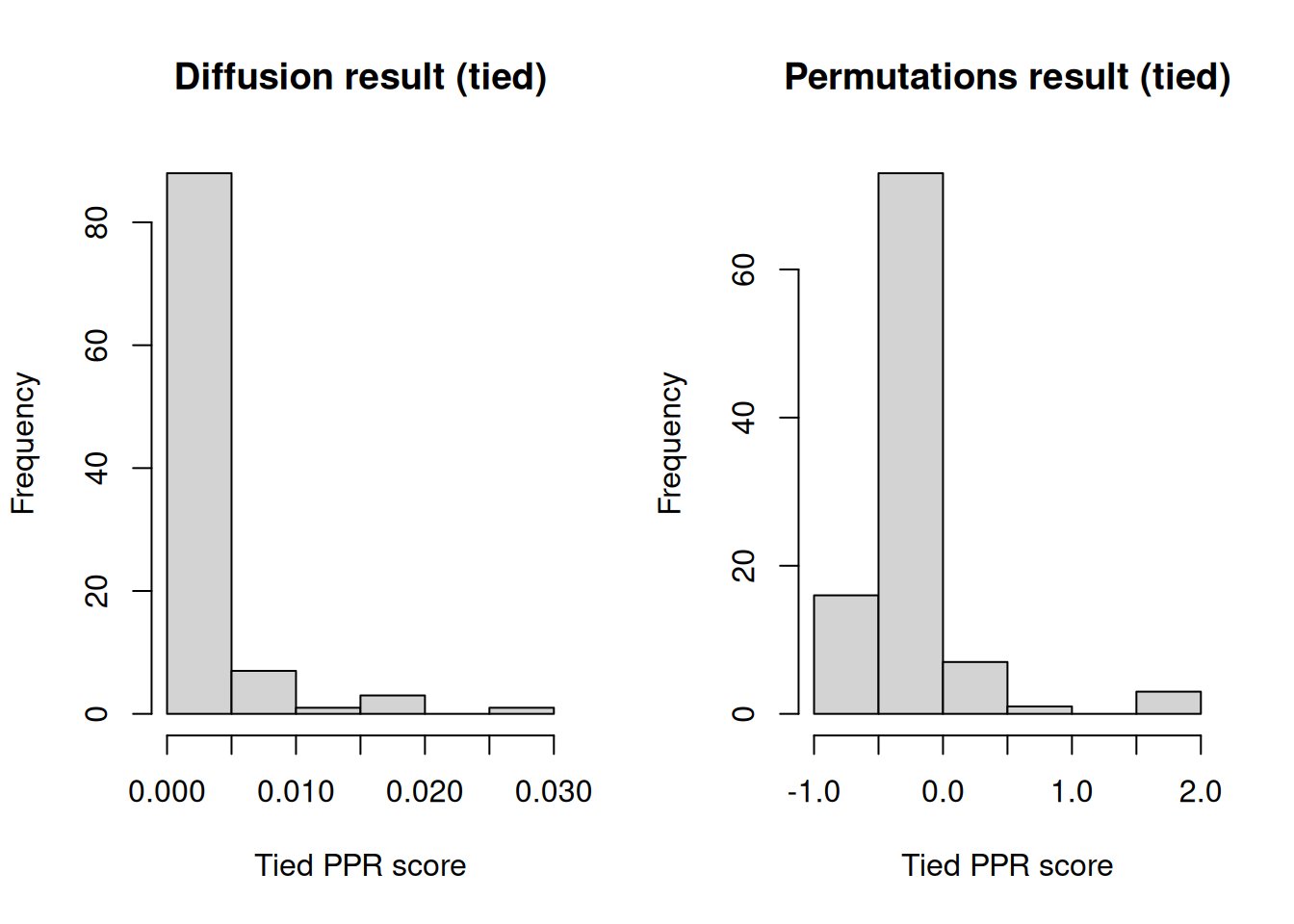
)Plotting the two:
diffusion_res <- get_diffusion_vector(diffusion_obj)
permutation_res <- get_diffusion_perms(diffusion_obj)

par(mfrow = c(1, 2))

hist(diffusion_res, xlab = "Tied PPR score", main = "Diffusion result (tied)")
hist(
  permutation_res,
  xlab = "Tied PPR score",
  main = "Permutations result (tied)"
)
You can again identify diffusion-heat privileged communities with the same methods. The function will automatically identify the type of diffusion you applied before. Let’s do this threshold based:
diffusion_obj <- community_detection(
  object = diffusion_obj,
  community_params = params_community_detection(
    min_nodes = 5L,
    threshold_type = "prop_based",
    min_seed_nodes = 1L
  )
)

results_v1 <- get_results(diffusion_obj)
head(results_v1)
#>    cluster_id node_id      ks_pval cluster_size seed_nodes_1 seed_nodes_2
#>        <char>  <char>        <num>        <int>        <int>        <int>
#> 1:  cluster_1  genes5 1.954153e-07           19            1            1
#> 2:  cluster_1  genes6 1.954153e-07           19            1            1
#> 3:  cluster_1 genes12 1.954153e-07           19            1            1
#> 4:  cluster_1 genes14 1.954153e-07           19            1            1
#> 5:  cluster_1 genes25 1.954153e-07           19            1            1
#> 6:  cluster_1 genes29 1.954153e-07           19            1            1
#>    diffusion_score seed_node_a seed_node_b
#>              <num>      <lgcl>      <lgcl>
#> 1:     0.026642185       FALSE       FALSE
#> 2:     0.003378515       FALSE       FALSE
#> 3:     0.006056165       FALSE       FALSE
#> 4:     0.006708816       FALSE       FALSE
#> 5:     0.002100994       FALSE       FALSE
#> 6:     0.001590163       FALSE       FALSE
Or p-value based:
diffusion_obj <- community_detection(
  object = diffusion_obj,
  community_params = params_community_detection(
    min_nodes = 2L,
    threshold_type = "pval_based",
    pval_threshold = 0.4, # Very high threshold here to identify any communities
    min_seed_nodes = 1L
  )
)

results_v2 <- get_results(diffusion_obj)
head(results_v2)
#>    cluster_id node_id     ks_pval cluster_size seed_nodes_1 seed_nodes_2
#>        <char>  <char>       <num>        <int>        <int>        <int>
#> 1:  cluster_1  genes2 0.005269523           19            1            2
#> 2:  cluster_1  genes5 0.005269523           19            1            2
#> 3:  cluster_1 genes17 0.005269523           19            1            2
#> 4:  cluster_1 genes21 0.005269523           19            1            2
#> 5:  cluster_1 genes59 0.005269523           19            1            2
#> 6:  cluster_1 genes87 0.005269523           19            1            2
#>    diffusion_score seed_node_a seed_node_b
#>              <num>      <lgcl>      <lgcl>
#> 1:     0.008902783       FALSE       FALSE
#> 2:     0.026642185       FALSE       FALSE
#> 3:     0.004129531        TRUE       FALSE
#> 4:     0.002532385       FALSE        TRUE
#> 5:     0.002532385       FALSE       FALSE
#> 6:     0.002532385       FALSE       FALSE
As you can appreciate, the diffusions can be used to identify more “influenced” parts of the network. If you want to transform the graphs into some embeddings for visualisations, also check out genewalkR which has very fast node2vec methods.