Doublet detection with bixverse • bixverse

Intro

Doublets - droplets containing two or more cells - are a common artefact in droplet-based single cell experiments. If left undetected, they masquerade as intermediate cell states or novel populations and quietly corrupt downstream analyses. This vignette demonstrates two doublet detection approaches available in bixverse and benchmarks them against ground truth calls from demuxlet, which identifies doublets via genetic variation across pooled donors.

bixverse provides two computational doublet detection methods:

Scrublet is a simulation-based approach (Wolock, et al., 2019). It generates synthetic doublets by averaging pairs of randomly selected cells, embeds both real and synthetic cells together, and scores each real cell by the proportion of its nearest neighbours that are synthetic. A bimodal score distribution is expected: singlets cluster near zero, doublets near one. A threshold on this score determines the final calls.
Boosted doublet detection takes a different angle. Rather than simulating doublets, it trains a gradient-boosted tree ensemble to distinguish real cells from synthetic doublets generated in the same way as Scrublet. The classifier produces a probability per cell, and doublet calls are derived from that probability. This can be more robust when the score distribution from Scrublet is not cleanly bimodal, though it introduces its own hyperparameters (and is slower).

Both methods are purely computational and work without genetic or hashing information. They complement experimental approaches like demuxlet, which require pooled donors or hashtag antibodies. They also have a failure mode if a large number of doublets dominates the original data.

library(bixverse)
library(data.table)

Loading the data

We use a PBMC data set with demuxlet ground truth calls. The demuxlet output classifies each barcode as a singlet (SNG) or doublet (DBL) (or ambiguous, but irrelevant for this situation), giving us something to benchmark against.

doublet_path <- download_demuxlet_pbmc()

tempdir_doublet <- file.path(tempdir(), "demuxlet_bixverse")
dir.create(tempdir_doublet, showWarnings = FALSE, recursive = TRUE)

demuxlet_data <- fread(file.path(doublet_path, "demuxlet_calls.tsv"))

table(demuxlet_data$Call)
#> 
#>   AMB   DBL   SNG 
#>    24  1565 13030

Load in the data into bixverse

sc_object <- SingleCells(dir_data = tempdir_doublet)

mtx_io_params <- get_cell_ranger_params(doublet_path)
mtx_io_params$cells_as_rows <- TRUE

sc_object <- load_mtx(
  object = sc_object,
  sc_mtx_io_param = mtx_io_params
)
#> Loading observations data from flat file into the DuckDB.
#> Loading variable data from flat file into the DuckDB.

sc_object
#> Single cell experiment (Single Cells).
#>   No cells (original): 14528
#>    To keep n: 14528
#>   No genes: 12622
#>   HVG calculated: FALSE
#>   PCA calculated: FALSE
#>   Other embeddings: none
#>   KNN generated: FALSE
#>   SNN generated: FALSE

We also define a small helper to compute precision, recall and F1 against the demuxlet calls.

doublet_metrics <- function(
  predicted,
  actual,
  pos_predicted = TRUE,
  pos_actual = "DBL"
) {
  tp <- sum(predicted == pos_predicted & actual == pos_actual)
  fp <- sum(predicted == pos_predicted & actual != pos_actual)
  fn <- sum(predicted != pos_predicted & actual == pos_actual)
  precision <- tp / (tp + fp)
  recall <- tp / (tp + fn)
  f1 <- 2 * (precision * recall) / (precision + recall)
  list(precision = precision, recall = recall, f1 = f1)
}

Doublet detection methods

Let’s check the two methods out and see how they behave

Scrublet

scrublet <- scrublet_sc(
  object = sc_object,
  scrublet_params = params_scrublet(
    expected_doublet_rate = 0.1
  )
)

scrublet
#> ScrubletRes: 14528 cells, 1753 doublets (12.1%)
#>   Threshold:              0.1852
#>   Detected doublet rate:  12.1%
#>   Detectable fraction:    87.3%
#>   Overall doublet rate:   13.8%
#>   Simulated doublets:     21792

The plot method shows the score distribution for observed and simulated cells. A clean separation between the two modes indicates the threshold is sensible.

plot(scrublet)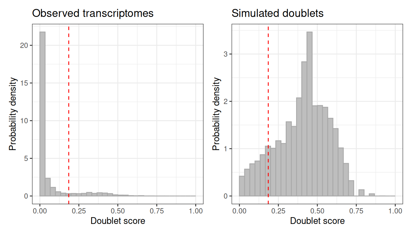

How does the automatic thresholding perform against the demuxlet ground truth?

scrublet_dt <- get_obs_data(scrublet)
scrublet_dt[, Barcode := get_cell_names(sc_object)]
scrublet_dt <- merge(scrublet_dt, demuxlet_data, by = "Barcode")

doublet_metrics(predicted = scrublet_dt$doublet, actual = scrublet_dt$Call)
#> $precision
#> [1] 0.6634341
#> 
#> $recall
#> [1] 0.745991
#> 
#> $f1
#> [1] 0.7022947

Manual threshold adjustment

The automatic threshold does not always land in the right place. If the score distribution suggests a different cut-off, call_doublets_manual lets you override it.

scrublet_adj <- call_doublets_manual(scrublet, threshold = 0.25)
#> Detected doublet rate = 10.0%
#> Estimated detectable doublet fraction = 80.4%
#> Overall doublet rate:
#>   Estimated = 12.4%

plot(scrublet_adj)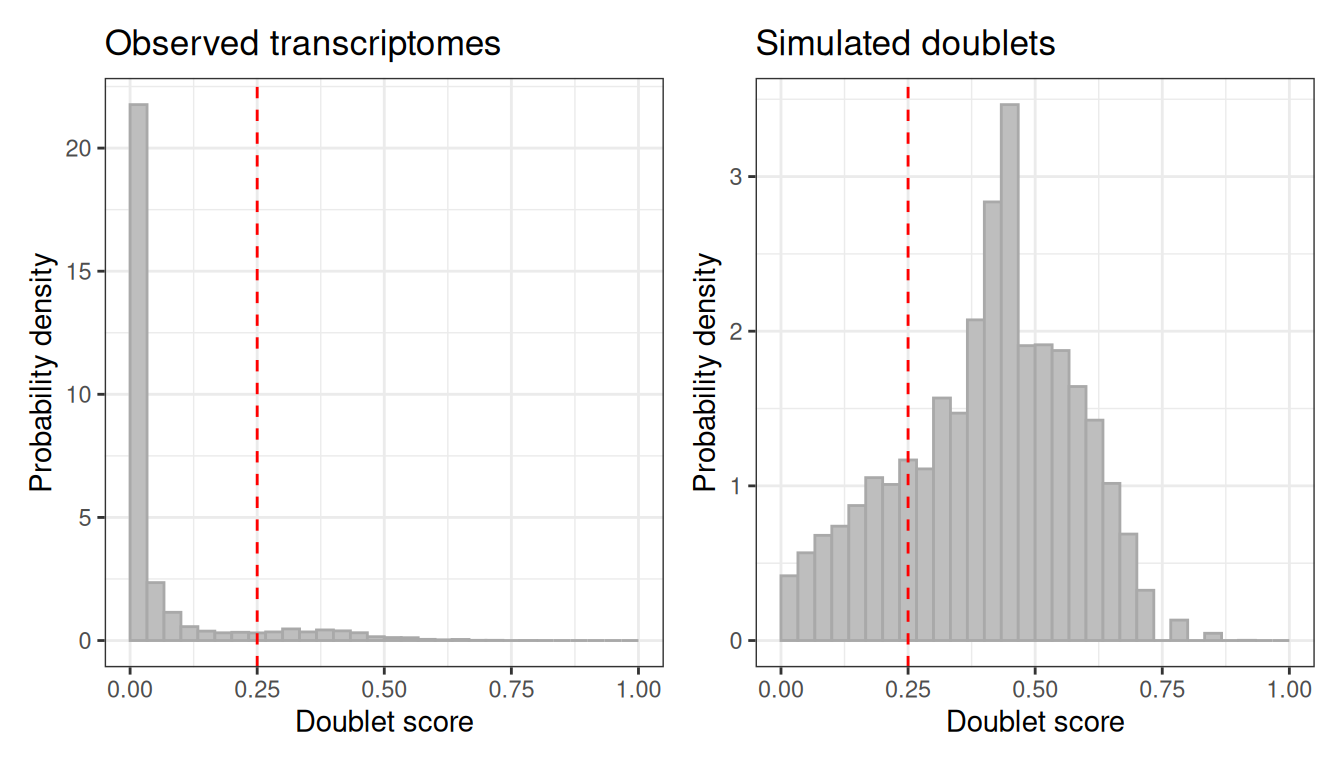

scrublet_adj_dt <- get_obs_data(scrublet_adj)
scrublet_adj_dt[, Barcode := get_cell_names(sc_object)]
scrublet_adj_dt <- merge(scrublet_adj_dt, demuxlet_data, by = "Barcode")

doublet_metrics(
  predicted = scrublet_adj_dt$doublet,
  actual = scrublet_adj_dt$Call
)
#> $precision
#> [1] 0.7015851
#> 
#> $recall
#> [1] 0.6529827
#> 
#> $f1
#> [1] 0.676412

We have made it worse here, but maybe there are cases where the scores are not very good. Compared to the original version, Otsu’s method is used to identify the perfect threshold, but it might fail in some situations.

Boosted doublet detection

The boosted approach trains a classifier to separate real cells from synthetic doublets. This can work better when the Scrublet score distribution is messy or unimodal. However, in this case we are running 25 iterations of the algorithm, which means 25x generation of synthetic doublets, re-normalisation, PCA, kNN, Louvain, classification. This makes this slower. We will be using "nndescent", one of the implemented kNN algorithms that can be faster at this data set size.

boosted_doublets <- doublet_detection_boost_sc(
  object = sc_object,
  boost_params = params_boost(knn = list(knn_method = "nndescent"))
)

boosted_doublets
#> BoostRes: 14528 cells, 1247 doublets (8.6%)
#>   Score range: [0.0057, 0.7240]

Let’s check how boosted works?

boosted_dt <- get_obs_data(boosted_doublets)
boosted_dt[, Barcode := get_cell_names(sc_object)]
boosted_dt <- merge(boosted_dt, demuxlet_data, by = "Barcode")

doublet_metrics(predicted = boosted_dt$doublet, actual = boosted_dt$Call)
#> $precision
#> [1] 0.7153168
#> 
#> $recall
#> [1] 0.5721616
#> 
#> $f1
#> [1] 0.6357805

Conclusion

Both methods can help to identify in a data-driven way doublets in your data. In this example, Scrublet performed better compared to boosted doublet detection, but you will have to see which one does better on your data. It can be worth running both and compare scores, expected doublet detections, etc. A longer idea will be to implement additionally also scDblFinder.

Clean up

unlink(tempdir_doublet, recursive = TRUE, force = TRUE)