library(bixverse)
library(data.table)
library(ggplot2)Batch correction with bixverse
Intro
Batch effects are systematic technical differences between experimental runs that can obscure genuine biological signal in single cell data. When datasets from multiple experiments, technologies, or laboratories are combined, cells tend to group by their source rather than by cell type. Batch correction methods aim to remove these technical artefacts whilst preserving biological variation.
bixverse provides three batch correction approaches, each with different trade-offs:
fastMNN (Haghverdi, et al., 2018) identifies mutual nearest neighbours across batches – pairs of cells from different batches that are each other’s closest match. Correction vectors are computed from these pairs and applied to align the embeddings. It is particularly effective when cell type composition differs across batches.
Harmony (Korsunsky, et al., 2019) operates on PCA embeddings using iterative soft clustering with diversity penalties. It assigns cells to clusters, estimates batch effects per cluster via ridge regression, and corrects the embedding. It tends to be fast and works well across a range of scenarios.
BBKNN (Polanski, et al., 2020) takes a fundamentally different approach. Rather than correcting an embedding, it constructs a batch-balanced k-nearest neighbour graph by building separate neighbour indices per batch. The corrected graph can then be used directly for clustering and visualisation.
bixverse also provides three metrics for assessing batch correction quality:
- kBET: tests whether neighbourhood batch proportions match global proportions (best for embedding-based methods).
- Batch ASW: measures batch separation in the embedding space (best for embedding-based methods).
- LISI: measures the effective number of batches per neighbourhood (works on any kNN graph).
Preparing the data
Loading the batches
We use two PBMC datasets (pbmc3k and pbmc4k) as a standard benchmark for batch correction. These come from the same tissue but differ in sequencing depth and cell counts, introducing a clear batch effect.
dir_data <- download_pbmc_batches()

tempdir_batch_cor <- file.path(tempdir(), "batch_cor_bixverse")
dir.create(tempdir_batch_cor, showWarnings = FALSE, recursive = TRUE)

h5ad_files <- list.files(dir_data)
h5ad_files <- h5ad_files[grepl(".h5ad", h5ad_files)]
h5ad_paths <- file.path(dir_data, h5ad_files)
names(h5ad_paths) <- c("pbmc3k", "pbmc4k")

h5_tasks <- prescan_h5ad_files(h5_paths = h5ad_paths)

sc_object <- SingleCells(dir_data = tempdir_batch_cor)

sc_object <- load_multi_h5ad(
  object = sc_object,
  prescan_result = h5_tasks,
  .verbose = TRUE
)
#> Loading observation data from h5ad files into DuckDB.
#> Loading variable data into DuckDB.
Quality control
Before batch correction, we filter out low-quality cells using mitochondrial gene proportions and library complexity metrics.
var <- get_sc_var(sc_object)

gs_of_interest <- list(
  MT = var[grepl("^MT-", symbol_tenx), gene_id],
  Ribo = var[grepl("^RPS|^RPL", symbol_tenx), gene_id]
)

sc_object <- gene_set_proportions_sc(
  sc_object,
  gs_of_interest,
  streaming = FALSE,
  .verbose = TRUE
)

qc_df <- sc_object[[c("cell_id", "lib_size", "nnz", "MT")]]

metrics <- list(
  log10_lib_size = log10(qc_df$lib_size),
  log10_nnz = log10(qc_df$nnz),
  MT = qc_df$MT
)
directions <- c(
  log10_lib_size = "twosided",
  log10_nnz = "twosided",
  MT = "above"
)

qc <- run_cell_qc(metrics, directions, threshold = 3)

qc
#> CellQc: 7040 cells, 1199 outliers (17.0%)
#> Metrics:
#>   - log10_lib_size: 450 outliers [lower = 3.07, upper = 3.93]
#>   - log10_nnz: 483 outliers [lower = 2.71, upper = 3.34]
#>   - MT: 728 outliers [upper = 0.05]
Let’s plot the metrics:
plots <- plot(qc, qc_df)

plots$log10_lib_size + plots$log10_nnz + plots$MT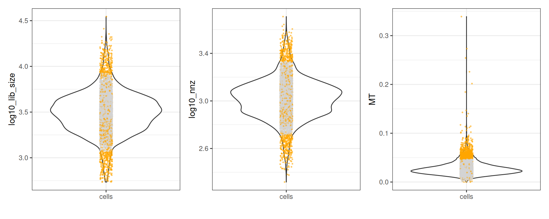
Set the cells to keep
sc_object[["outlier"]] <- qc$combined
cells_to_keep <- qc_df[!qc$combined, cell_id]
sc_object <- set_cells_to_keep(sc_object, cells_to_keep)
Pre-processing
Standard pre-processing: HVG selection, PCA, and neighbour computation.
sc_object <- find_hvg_sc(
  object = sc_object,
  hvg_no = 2000L,
  .verbose = TRUE
)

sc_object <- calculate_pca_sc(
  object = sc_object,
  no_pcs = 30L
)
#> Using dense SVD solving on scaled data on 2000 HVG.

sc_object <- find_neighbours_sc(
  object = sc_object,
  neighbours_params = params_sc_neighbours(
    knn = list(knn_method = "exhaustive")
  )
)
#>
#> Generating sNN graph (full: FALSE).
#> Transforming sNN data to igraph.
Comparing the different methods
Let’s check out the different methods and how they behave.
Uncorrected data
Before applying any correction, we can visualise the batch effect and compute baseline metrics.
sc_object <- tsne_sc(object = sc_object)
#> Running t-SNE.
#> Using provided kNN graph.

tsne_dt_pre <- as.data.table(
  get_embedding(sc_object, "tsne"),
  keep.rownames = "cell_id"
)[, batch := sc_object[["sample"]]]
tSNE plot (tSNE’s usually look prettier… It’s anyway not a good way to assess batch effect correction, so at least let’s make it pleasant on the eye).
ggplot(tsne_dt_pre, aes(x = tsne_1, y = tsne_2)) +
  geom_point(aes(colour = as.factor(batch)), alpha = 0.5, size = 0.5) +
  labs(
    x = "tSNE1",
    y = "tSNE2",
    title = "Before batch correction",
    colour = "Batch:"
  ) +
  theme_bw()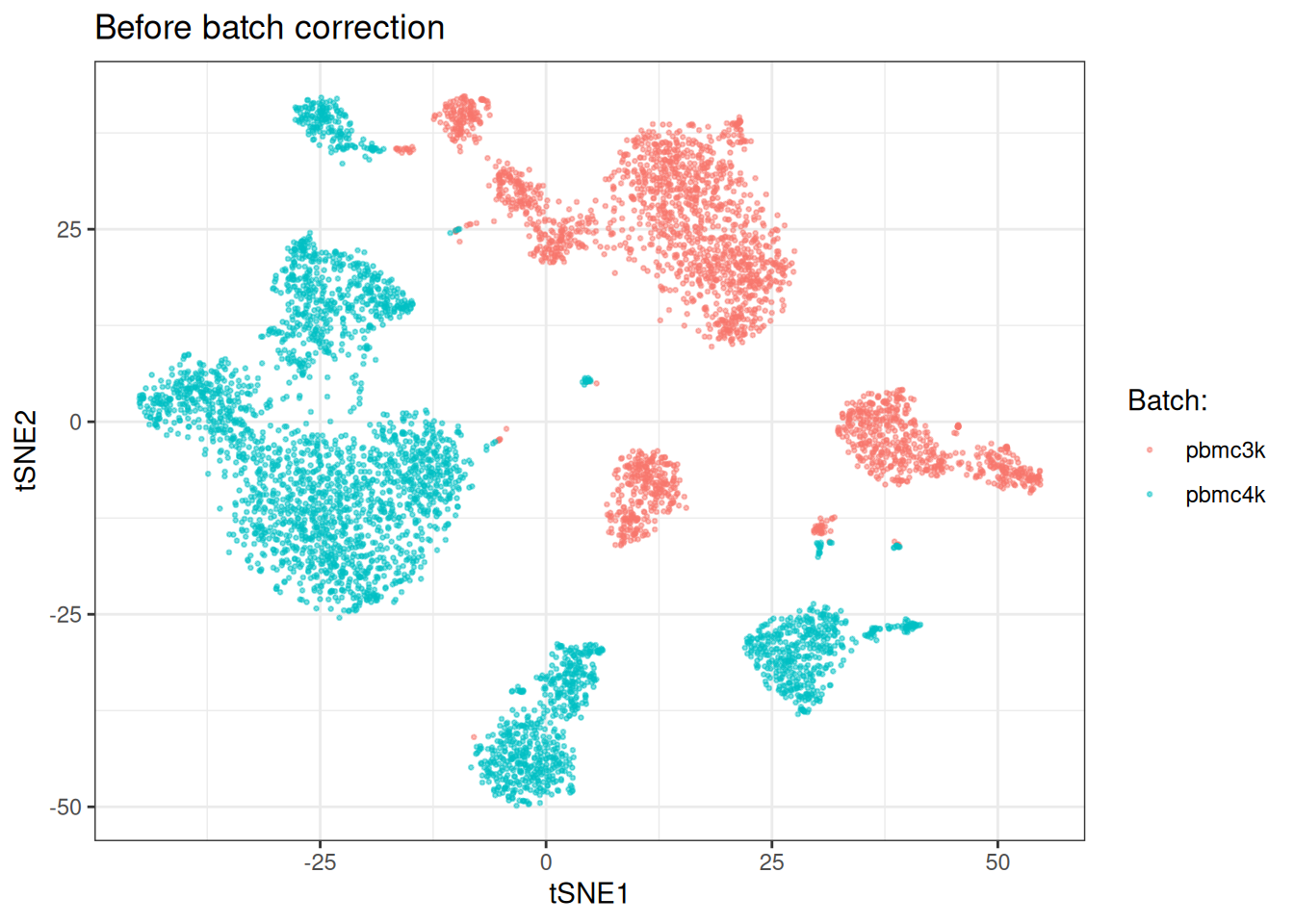
Batch correction stats:
kbet_score_prior <- calculate_kbet_sc(sc_object, batch_column = "sample")
asw_score_prior <- calculate_batch_asw_sc(sc_object, batch_column = "sample")
lisi_score_prior <- calculate_batch_lisi_sc(sc_object, batch_column = "sample")

kbet_score_prior
#> kBET Scores
#>   Cells: 5841 | Batches: 2 | Threshold: 0.050
#>   Rejection rate:      0.9882 (5772 / 5841)
#>   Mean Chi-Square:     12.8160 (expected under H0: 1)
#>   Median Chi-Square:   8.7578
asw_score_prior
#> Batch Silhouette Width
#>   Cells: 5000 | Batches: 2
#>   Mean ASW:    0.1103 (0 = perfect mixing, 1 = separated)
#>   Median ASW:  0.1213
lisi_score_prior
#> Batch LISI Scores
#>   Cells: 5841 | Batches: 2
#>   Mean LISI:    1.0130 (1 = no mixing, 2 = perfect mixing)
#>   Median LISI:  1.0000
The high kBET rejection rate and mean chi-square well above the expected value of 1 confirm a substantial batch effect. LISI scores also indicate very poor batch matching and the tSNE shows clear separation by batch.
fastMNN
fastMNN works on batch-aware HVGs and produces a corrected embedding. It identifies mutual nearest neighbours across batches to compute correction vectors. For it to work best, we need the batch-aware HVGs. We will calculate these, provide them to fastMNN (which regenerates the PCA embedding based on the batch-aware HVG) and run then the actual algorithm
batch_aware_hvg <- find_hvg_batch_aware_sc(
  object = sc_object,
  batch_column = "sample"
)

sc_object <- fast_mnn_sc(
  object = sc_object,
  batch_hvg_genes = batch_aware_hvg$hvg_genes,
  batch_column = "sample"
)

sc_object <- find_neighbours_sc(
  object = sc_object,
  embd_to_use = "mnn",
  neighbours_params = params_sc_neighbours(
    knn = list(knn_method = "exhaustive")
  )
)
#>
#> Generating sNN graph (full: FALSE).
#> Transforming sNN data to igraph.
kbet_score_post_mnn <- calculate_kbet_sc(
  sc_object,
  batch_column = "sample"
)
asw_score_post_mnn <- calculate_batch_asw_sc(
  sc_object,
  embd_to_use = "mnn",
  batch_column = "sample"
)
lisi_score_post_mnn <- calculate_batch_lisi_sc(
  sc_object,
  batch_column = "sample"
)

kbet_score_post_mnn
#> kBET Scores
#>   Cells: 5841 | Batches: 2 | Threshold: 0.050
#>   Rejection rate:      0.3489 (2038 / 5841)
#>   Mean Chi-Square:     3.5932 (expected under H0: 1)
#>   Median Chi-Square:   3.6444
asw_score_post_mnn
#> Batch Silhouette Width
#>   Cells: 5000 | Batches: 2
#>   Mean ASW:    0.0186 (0 = perfect mixing, 1 = separated)
#>   Median ASW:  0.0428
lisi_score_post_mnn
#> Batch LISI Scores
#>   Cells: 5841 | Batches: 2
#>   Mean LISI:    1.4450 (1 = no mixing, 2 = perfect mixing)
#>   Median LISI:  1.4706
We can see clear improvements across all scores. Lower kBET scores, better mean AWS scores and LISI scores also closer to 2 (i.e., number of batches).
sc_object <- tsne_sc(object = sc_object)
#> Running t-SNE.
#> Using provided kNN graph.

tsne_dt_mnn <- as.data.table(
  get_embedding(sc_object, "tsne"),
  keep.rownames = "cell_id"
)[, batch := sc_object[["sample"]]]
ggplot(tsne_dt_mnn, aes(x = tsne_1, y = tsne_2)) +
  geom_point(aes(colour = as.factor(batch)), alpha = 0.5, size = 0.5) +
  labs(
    x = "tSNE1",
    y = "tSNE2",
    title = "fastMNN batch correction",
    colour = "Batch:"
  ) +
  theme_bw()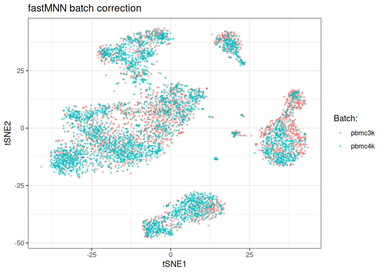
Also, visually the batches get mixed now.
Harmony
Harmony operates on the PCA embedding directly. The number of clusters is auto-determined from the dataset size (capped at 200) when left as NULL.
sc_object <- harmony_sc(
  object = sc_object,
  batch_column = "sample",
  harmony_params = params_sc_harmony()
)
#>  Auto-determined number of Harmony clusters: 195

sc_object <- find_neighbours_sc(
  object = sc_object,
  embd_to_use = "harmony",
  neighbours_params = params_sc_neighbours(
    knn = list(knn_method = "exhaustive")
  )
)
#>
#> Generating sNN graph (full: FALSE).
#> Transforming sNN data to igraph.
Let’s calculate the batch correction-related scores
kbet_score_post_harmony <- calculate_kbet_sc(
  sc_object,
  batch_column = "sample"
)
asw_score_post_harmony <- calculate_batch_asw_sc(
  sc_object,
  embd_to_use = "harmony",
  batch_column = "sample"
)
lisi_score_post_harmony <- calculate_batch_lisi_sc(
  sc_object,
  batch_column = "sample"
)

kbet_score_post_harmony
#> kBET Scores
#>   Cells: 5841 | Batches: 2 | Threshold: 0.050
#>   Rejection rate:      0.1481 (865 / 5841)
#>   Mean Chi-Square:     2.1294 (expected under H0: 1)
#>   Median Chi-Square:   1.5425
asw_score_post_harmony
#> Batch Silhouette Width
#>   Cells: 5000 | Batches: 2
#>   Mean ASW:    0.0201 (0 = perfect mixing, 1 = separated)
#>   Median ASW:  0.0353
lisi_score_post_harmony
#> Batch LISI Scores
#>   Cells: 5841 | Batches: 2
#>   Mean LISI:    1.5908 (1 = no mixing, 2 = perfect mixing)
#>   Median LISI:  1.6423
Also here, we observe improvements across the board.
sc_object <- tsne_sc(object = sc_object)
#> Running t-SNE.
#> Using provided kNN graph.

tsne_dt_harmony <- as.data.table(
  get_embedding(sc_object, "tsne"),
  keep.rownames = "cell_id"
)[, batch := sc_object[["sample"]]]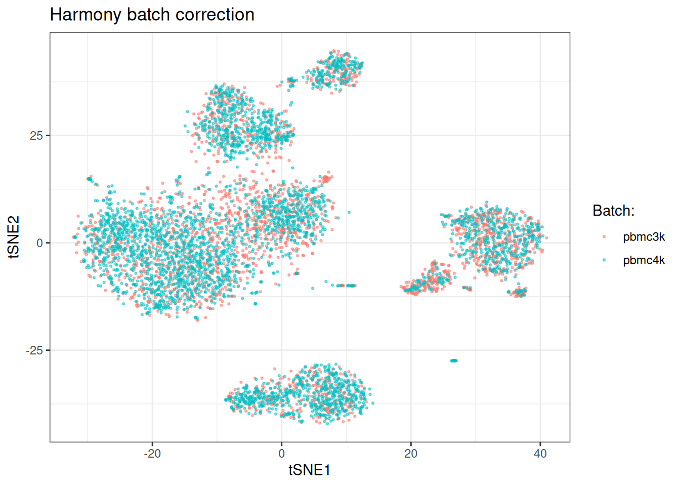
BBKNN
BBKNN constructs a batch-balanced kNN graph rather than correcting an embedding. The key parameter is neighbours_within_batch, which controls how many neighbours are found per batch. Setting no_neighbours_to_keep below the total generated neighbours (here 10 from 2 batches = 20 total) ensures the distance-based filtering introduces genuine variation, making downstream metrics informative.
Note that kBET and ASW are not well suited for evaluating BBKNN: kBET compares neighbourhood proportions against global proportions, which BBKNN manipulates by design, and ASW requires an embedding. LISI on the stored kNN is the most appropriate metric here.
sc_object <- bbknn_sc(
  object = sc_object,
  batch_column = "sample",
  no_neighbours_to_keep = 15L,
  bbknn_params = params_sc_bbknn(neighbours_within_batch = 10L)
)
#> Warning in `method(bbknn_sc, bixverse::SingleCells)`(object = <object>, : Prior
#> kNN matrix found. Will be overwritten.
#> Running BBKNN algorithm.
#> Generating graph based on BBKNN connectivities. Weights will be based on the connectivities and not shared nearest neighbour calculations.
kbet_score_post_bbknn <- calculate_kbet_sc(
  sc_object,
  batch_column = "sample"
)
lisi_score_post_bbknn <- calculate_batch_lisi_sc(
  sc_object,
  batch_column = "sample"
)

kbet_score_post_bbknn
#> kBET Scores
#>   Cells: 5841 | Batches: 2 | Threshold: 0.050
#>   Rejection rate:      0.0000 (0 / 5841)
#>   Mean Chi-Square:     3.1228 (expected under H0: 1)
#>   Median Chi-Square:   3.1228
lisi_score_post_bbknn
#> Batch LISI Scores
#>   Cells: 5841 | Batches: 2
#>   Mean LISI:    1.7999 (1 = no mixing, 2 = perfect mixing)
#>   Median LISI:  1.8000
sc_object <- tsne_sc(object = sc_object)
#> Running t-SNE.
#> Using provided kNN graph.

tsne_dt_bbknn <- as.data.table(
  get_embedding(sc_object, "tsne"),
  keep.rownames = "cell_id"
)[, batch := sc_object[["sample"]]]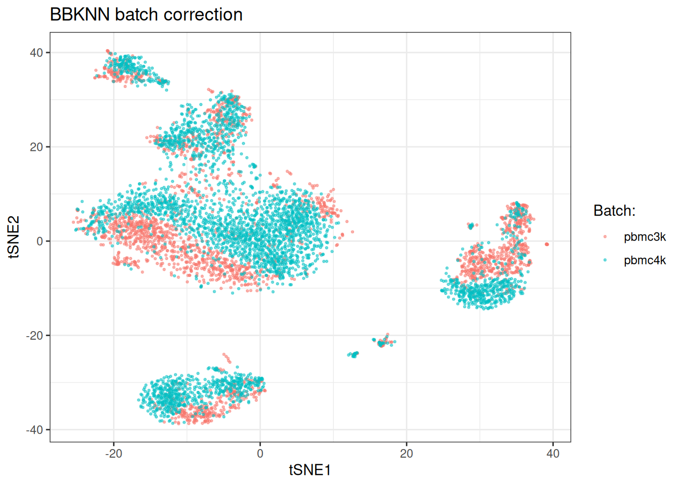
Choosing a method
There is no universally best batch correction method. Some practical guidance:
Harmony is a good default. It is fast, operates on the PCA embedding directly, and handles multiple batch variables simultaneously. It tends to work well when batch effects are moderate and cell type composition is broadly similar across batches.
fastMNN is worth considering when cell type composition differs substantially across batches. The mutual nearest neighbour approach is less sensitive to this because it only aligns cells that have a plausible biological match in another batch.
BBKNN is useful when you want to avoid modifying the embedding at all. The batch-balanced graph can be passed directly to graph-based clustering algorithms. It is the lightest-touch approach but provides less control over the degree of correction.
In practice, running multiple methods and looking at quantitative metrics is the most reliable approach. No single metric captures everything – kBET and ASW measure different aspects of embedding-based correction, and LISI is most informative for graph-based methods. UMAPs and tSNE assessments should be taken with a big pinch of salt, see Chari, et al.. Admittedly, they do look pretty however.
Clean up
unlink(tempdir_batch_cor, recursive = TRUE, force = TRUE)