library(bixverse)
library(ggplot2)
library(data.table)Analysing PBMCs with bixverse
Intro
This vignette walks through a standard single cell analysis on the PBMC3k data set using bixverse. If you have not read the design choices and the introductory vignette, please do so first; this vignette assumes familiarity with how the SingleCells class, on-disk storage and cells-to-keep logic work.
Loading the data
We start by downloading the PBMC3k data set bundled with the package and loading it via Cell Ranger-style MTX I/O.
pbmc3k_path <- bixverse:::download_pbmc3k()

tempdir_pbmc <- tempdir()

sc_object <- SingleCells(dir_data = tempdir_pbmc)

mtx_io_params <- get_cell_ranger_params(pbmc3k_path)

sc_object <- load_mtx(
  object = sc_object,
  sc_mtx_io_param = mtx_io_params,
  streaming = FALSE,
  .verbose = TRUE
)
#> Loading observations data from flat file into the DuckDB.
#> Loading variable data from flat file into the DuckDB.

sc_object
#> Single cell experiment (Single Cells).
#>   No cells (original): 2700
#>    To keep n: 2700
#>   No genes: 11139
#>   HVG calculated: FALSE
#>   PCA calculated: FALSE
#>   Other embeddings: none
#>   KNN generated: FALSE
#>   SNN generated: FALSE
Let’s have a quick look at the variable table. The column names from the MTX files are not always informative, so we rename the gene symbol column to something sensible and set up mappings between Ensembl IDs and symbols.
var <- get_sc_var(sc_object)

head(var)
#>    gene_idx         gene_id   column1 no_cells_exp
#>       <num>          <char>    <char>        <int>
#> 1:        1 ENSG00000225880 LINC00115           18
#> 2:        2 ENSG00000188976     NOC2L          258
#> 3:        3 ENSG00000188290      HES4          145
#> 4:        4 ENSG00000187608     ISG15         1206
#> 5:        5 ENSG00000131591  C1orf159           24
#> 6:        6 ENSG00000186891  TNFRSF18           92

setnames_sc(
  object = sc_object,
  table = "var",
  old = "column1",
  new = "gene_symbol"
)

var <- get_sc_var(sc_object)

head(var)
#>    gene_idx         gene_id gene_symbol no_cells_exp
#>       <num>          <char>      <char>        <int>
#> 1:        1 ENSG00000225880   LINC00115           18
#> 2:        2 ENSG00000188976       NOC2L          258
#> 3:        3 ENSG00000188290        HES4          145
#> 4:        4 ENSG00000187608       ISG15         1206
#> 5:        5 ENSG00000131591    C1orf159           24
#> 6:        6 ENSG00000186891    TNFRSF18           92

ensembl_to_symbol <- setNames(var$gene_symbol, var$gene_id)
symbol_to_ensembl <- setNames(var$gene_id, var$gene_symbol)
Quality control
Gene set proportions
A typical first step is computing the proportion of counts mapping to mitochondrial and ribosomal genes per cell. These are added directly to the obs table in the DuckDB.
gs_of_interest <- list(
  MT = var[grepl("^MT-", gene_symbol), gene_id],
  Ribo = var[grepl("^RPS|^RPL", gene_symbol), gene_id]
)

sc_object <- gene_set_proportions_sc(
  sc_object,
  gs_of_interest,
  streaming = FALSE,
  .verbose = TRUE
)

sc_object[[1:5L]]
#>    cell_idx          cell_id   nnz lib_size to_keep          MT      Ribo
#>       <num>           <char> <num>    <num>  <lgcl>       <num>     <num>
#> 1:        1 AAACATACAACCAC-1   778     2418    TRUE 0.030190241 0.4371381
#> 2:        2 AAACATTGAGCTAC-1  1346     4896    TRUE 0.037990198 0.4246323
#> 3:        3 AAACATTGATCAGC-1  1126     3144    TRUE 0.008905852 0.3171120
#> 4:        4 AAACCGTGCTTCCG-1   953     2632    TRUE 0.017477203 0.2431611
#> 5:        5 AAACCGTGTATGCG-1   520      979    TRUE 0.012257406 0.1491318
As we can see we now have MT and Ribo as columns in the obs table.
MAD outlier detection
We use per-cell QC metrics and MAD-based outlier detection to flag problematic cells. The run_cell_qc function returns a CellQc object that carries the metrics, per-metric outlier calls and a combined outlier vector.
qc_df <- sc_object[[c("cell_id", "lib_size", "nnz", "MT")]]

metrics <- list(
  log10_lib_size = log10(qc_df$lib_size),
  log10_nnz = log10(qc_df$nnz),
  MT = qc_df$MT
)

directions <- c(
  log10_lib_size = "twosided",
  log10_nnz = "twosided",
  MT = "above"
)

qc <- run_cell_qc(metrics, directions, threshold = 3)

qc
#> CellQc: 2700 cells, 537 outliers (19.9%)
#> Metrics:
#>   - log10_lib_size: 336 outliers [lower = 3.05, upper = 3.64]
#>   - log10_nnz: 383 outliers [lower = 2.70, upper = 3.12]
#>   - MT: 201 outliers [upper = 0.04]
The CellQc class has a plot method that produces violin plots with outliers highlighted.
plots <- plot(qc, qc_df)

plots$log10_lib_size + plots$log10_nnz + plots$MT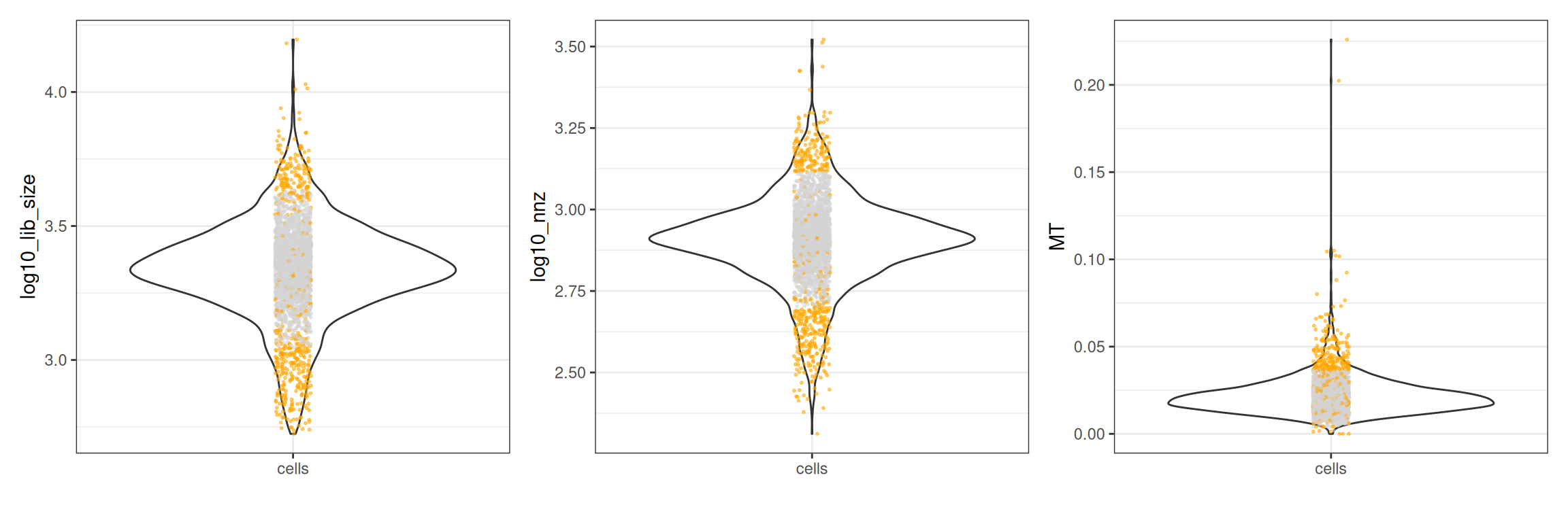
Filtering cells
We store the outlier flag in the obs table and then set the cells to keep. From this point on, all downstream methods (HVG selection, PCA, etc.) will only operate on the retained cells.
sc_object[["outlier"]] <- qc$combined

cells_to_keep <- qc_df[!qc$combined, cell_id]

sc_object <- set_cells_to_keep(sc_object, cells_to_keep)

sc_object
#> Single cell experiment (Single Cells).
#>   No cells (original): 2700
#>    To keep n: 2163
#>   No genes: 11139
#>   HVG calculated: FALSE
#>   PCA calculated: FALSE
#>   Other embeddings: none
#>   KNN generated: FALSE
#>   SNN generated: FALSE
Feature selection, PCA and neighbours
With QC done, we move through the standard pipeline: highly variable gene selection, PCA, and nearest neighbour computation.
sc_object <- find_hvg_sc(
  object = sc_object,
  hvg_no = 2000L,
  .verbose = TRUE
)

sc_object <- calculate_pca_sc(
  object = sc_object,
  no_pcs = 30L,
  sparse_svd = TRUE
)
#> Using sparse SVD solving on scaled data on 2000 HVG.

# the data is so tiny that exhaustive kNN search is faster than building
# an approximate nearest neighbour index
sc_object <- find_neighbours_sc(
  object = sc_object,
  neighbours_params = params_sc_neighbours(
    knn = list(knn_method = "exhaustive")
  )
)
#>
#> Generating sNN graph (full: FALSE).
#> Transforming sNN data to igraph.
Clustering and marker detection
Leiden clustering followed by differential gene expression across all clusters.
sc_object <- find_clusters_sc(sc_object, res = 1.5, name = "leiden_clusters")

all_markers <- find_all_markers_sc(
  object = sc_object,
  column_of_interest = "leiden_clusters"
)
#> Processing group 1 out of 7.
#> Processing group 2 out of 7.
#> Processing group 3 out of 7.
#> Processing group 4 out of 7.
#> Processing group 5 out of 7.
#> Processing group 6 out of 7.
#> Processing group 7 out of 7.

all_markers[, gene_symbol := ensembl_to_symbol[gene_id]]

head(all_markers[fdr <= 0.05][order(-abs(lfc))])
#>      grp         gene_id      lfc     prop1      prop2 z_scores      p_values
#>    <num>          <char>    <num>     <num>      <num>    <num>         <num>
#> 1:     6 ENSG00000163220 4.174770 0.9887324 0.20077434 29.09827 1.887722e-186
#> 2:     7 ENSG00000105374 4.156168 1.0000000 0.25049117 18.50890  8.752290e-77
#> 3:     6 ENSG00000090382 4.081069 1.0000000 0.51050884 29.66810 9.907717e-194
#> 4:     7 ENSG00000115523 3.934315 0.9527559 0.13654225 17.52567  4.562691e-69
#> 5:     6 ENSG00000143546 3.663987 0.9718310 0.11504425 28.62794 1.508612e-180
#> 6:     7 ENSG00000100453 3.544770 0.9842520 0.06974459 18.39899  6.691597e-76
#>              fdr gene_symbol
#>            <num>      <char>
#> 1: 4.275690e-183      S100A9
#> 2:  3.963037e-73        NKG7
#> 3: 4.488196e-190         LYZ
#> 4:  5.164966e-66        GNLY
#> 5: 2.278005e-177      S100A8
#> 6:  1.514978e-72        GZMB
Visualisation
Dimensionality reduction
Let us run quickly UMAP and tSNE.
We can pull the embeddings back into data.tables and plot them (longer term, the idea will be to provide plotting helpers in bixverse.plots). The obs columns can be appended directly.
umap_dt <- as.data.table(
  get_embedding(sc_object, "umap"),
  keep.rownames = "cell_id"
)[, leiden_clusters := sc_object[["leiden_clusters"]]]

ggplot(umap_dt, aes(x = umap_1, y = umap_2)) +
  geom_point(aes(colour = as.factor(leiden_clusters)), size = 0.5) +
  theme_bw() +
  labs(colour = "Leiden cluster")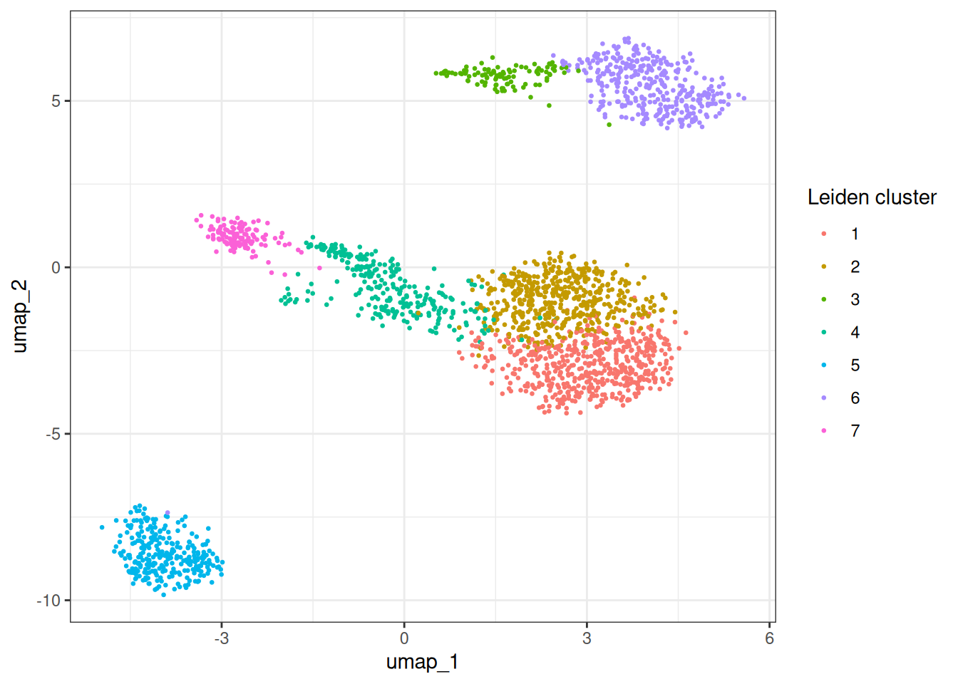
Let’s check out tSNE
tsne_dt <- as.data.table(
  get_embedding(sc_object, "tsne"),
  keep.rownames = "cell_id"
)[, leiden_clusters := sc_object[["leiden_clusters"]]]

ggplot(tsne_dt, aes(x = tsne_1, y = tsne_2)) +
  geom_point(aes(colour = as.factor(leiden_clusters)), size = 0.5) +
  theme_bw() +
  labs(colour = "Leiden cluster")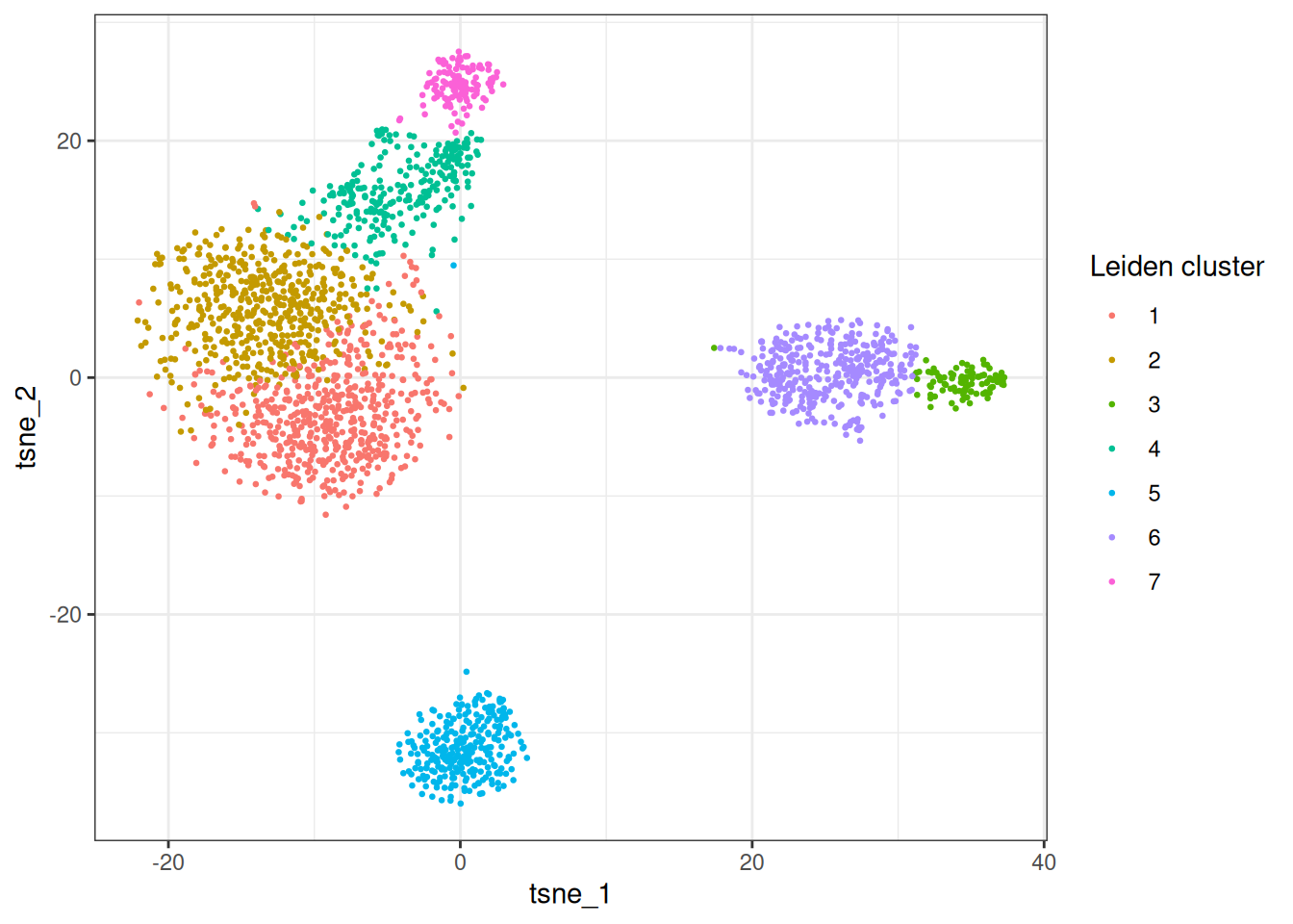
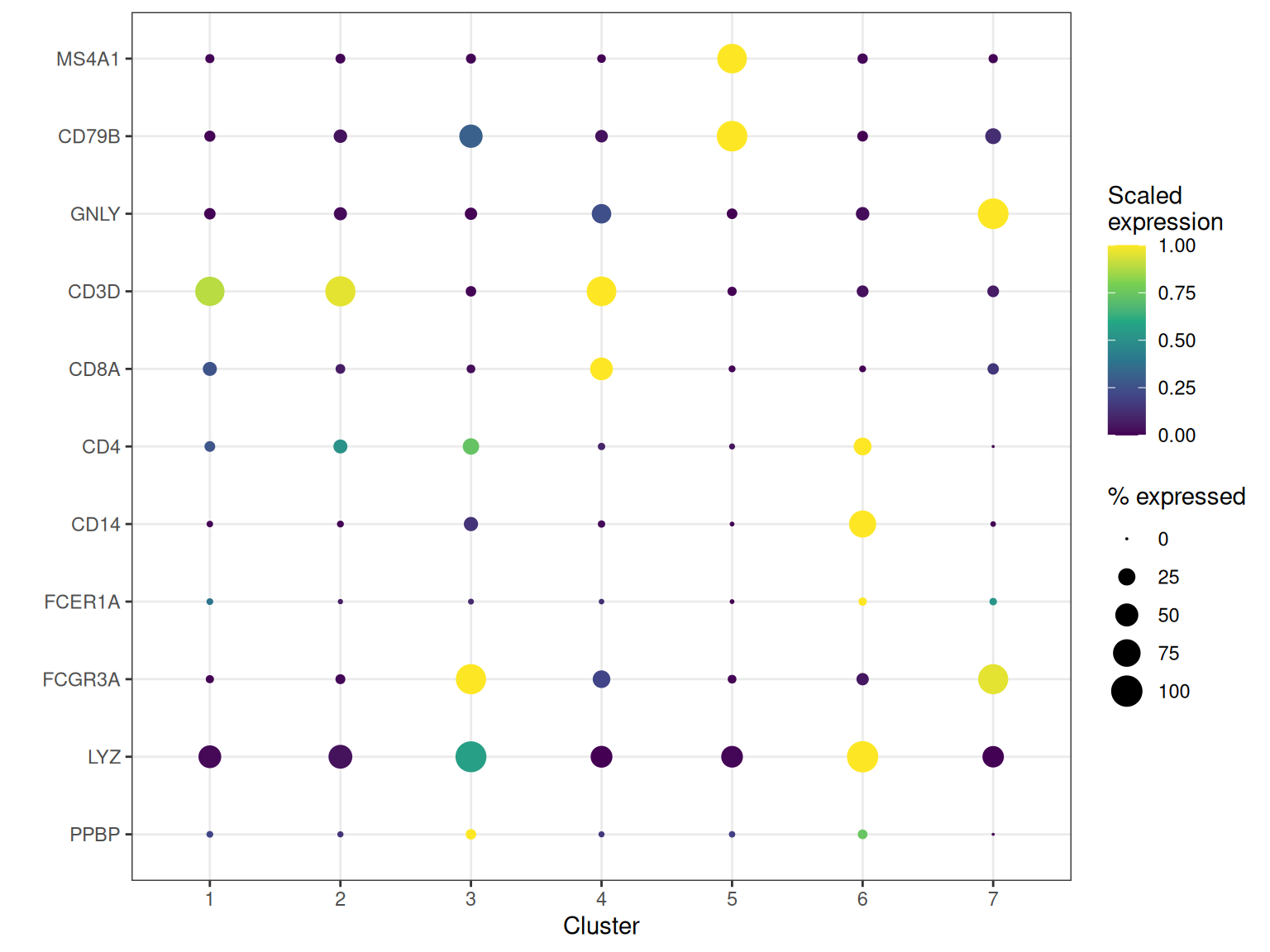
Dot plots
Dot plots are a standard way to visualise marker gene expression across clusters. The extract_dot_plot_data method handles the Rust-level extraction, grouping statistics and optional min-max scaling in one call.
cell_markers <- c(
  "MS4A1",
  "CD79B",
  "GNLY",
  "CD3D",
  "CD8A",
  "CD4",
  "CD14",
  "FCER1A",
  "FCGR3A",
  "LYZ",
  "PPBP"
)

features <- symbol_to_ensembl[cell_markers]

dot_dt <- extract_dot_plot_data(
  object = sc_object,
  features = features,
  grouping_variable = "leiden_clusters",
  scale_exp = TRUE
)

dot_dt[, gene_symbol := ensembl_to_symbol[as.character(gene)]]
dot_dt[, gene_symbol := factor(gene_symbol, levels = rev(cell_markers))]

ggplot(dot_dt, aes(x = group, y = gene_symbol)) +
  geom_point(aes(size = pct_exp, colour = scaled_exp)) +
  scale_colour_viridis_c() +
  scale_size_continuous(range = c(0, 6)) +
  theme_bw() +
  labs(
    size = "% expressed",
    colour = "Scaled\nexpression",
    x = "Cluster",
    y = ""
  )
Per-cell gene expression
For feature plots or other per-cell visualisations, extract_gene_expression returns a long data.table with one row per cell and columns for each requested gene, plus any obs metadata you need.
expr_dt <- extract_gene_expression(
  object = sc_object,
  features = symbol_to_ensembl[c("CD14", "MS4A1", "CD3E")],
  obs_cols = "leiden_clusters"
)

# attach UMAP coordinates
umap_embd <- as.data.table(
  get_embedding(sc_object, "umap"),
  keep.rownames = "cell_id"
)

plot_dt <- merge(expr_dt, umap_embd, by = "cell_id")

# melt to long for faceting
gene_cols <- symbol_to_ensembl[c("CD14", "MS4A1", "CD3E")]

plot_long <- melt(
  plot_dt,
  id.vars = c("cell_id", "umap_1", "umap_2"),
  measure.vars = gene_cols,
  variable.name = "gene",
  value.name = "expression"
)
plot_long[, gene_symbol := ensembl_to_symbol[as.character(gene)]]

ggplot(plot_long, aes(x = umap_1, y = umap_2)) +
  geom_point(aes(colour = expression), size = 0.3) +
  scale_colour_viridis_c() +
  facet_wrap(~gene_symbol) +
  theme_bw() +
  labs(colour = "log1p\nexpression")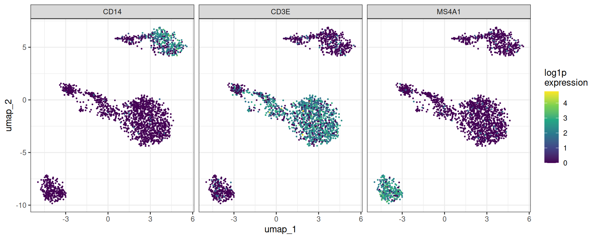
Clean up
unlink(tempdir_pbmc, recursive = TRUE, force = TRUE)