if (!requireNamespace("fgsea", quietly = TRUE)) {
  BiocManager::install("fgsea")
}
if (!requireNamespace("msigdbr", quietly = TRUE)) {
  install.packages("msigdbr")
}
library(bixverse)
library(data.table)
library(magrittr)Gene Set Enrichment Methods
Gene Set Enrichment Methods in bixverse
This vignette shows you how to use the gene set enrichment methods implemented in bixverse.
Intro
Gene set enrichment analysis sits at the heart of most functional genomics workflows. Given a set of genes of interest (or a ranked list of all measured genes) you want to know which biological processes, pathways, or molecular functions are over-represented relative to what you would expect by chance. bixverse provides Rust-accelerated implementations of the two dominant paradigms for this, along with gene ontology-aware variants of each.
Over-representation analysis (ORA) via the hypergeometric test asks: given that I have drawn genes from a universe of , and of those belong to a particular gene set, is the overlap of larger than expected? This is fast and interpretable, but requires a discrete gene list — typically genes passing some fold-change and significance threshold. The choice of threshold and universe can substantially affect results, which is a known limitation of the approach.
Gene Set Enrichment Analysis (GSEA) sidesteps this by working with a continuously ranked list of all measured genes, asking whether the members of a gene set are systematically concentrated towards the top or bottom of the ranking. This avoids arbitrary thresholding and tends to be more sensitive to coordinated but modest shifts in expression, at the cost of being more computationally demanding and less straightforward to interpret.
A practical complication with both approaches is the redundancy of the Gene Ontology (GO). The GO is a directed acyclic graph: a significant hit on a specific term (e.g., “mitochondrial complex I assembly”) will typically also produce significant hits on all of its ancestor terms (e.g., “oxidative phosphorylation”, “metabolic process”), most of which add no new information. bixverse provides two strategies for dealing with this: the elimination method of Adrian et al., which propagates signal up the DAG while removing explained genes, and a post-hoc simplification approach based on Wang semantic similarity, which collapses redundant terms after running a standard enrichment.
All methods are implemented in Rust and exposed via extendr. The performance gains relative to existing R implementations range from modest (~20% faster for GSEA relative to fgsea’s Rcpp implementation) to substantial: the parallelised hypergeometric test over large gene set libraries can be orders of magnitude faster than a naive R loop.
Hypergeometric tests
bixverse implements the standard hypergeometric over-representation test. In this example we load the Hallmark gene sets from msigdbr and construct a named list, which is the expected input format throughout bixverse for gene set analyses.
To test a single target gene set, use gse_hypergeometric. The gene universe defaults to the union of all genes represented in the gene_set_list if not provided explicitly. This is usually reasonable but worth checking if your assay covers a non-standard set of genes. FDR threshold and minimum overlap are also configurable.
results <- gse_hypergeometric(
  target_genes = target_genes_1,
  gene_set_list = h_gene_sets_ls
)

head(results)
#>              gene_set_name odds_ratios        pvals          fdr  hits
#>                     <char>       <num>        <num>        <num> <num>
#> 1: HALLMARK_MYC_TARGETS_V2   170.67009 5.919144e-41 2.959572e-39    27
#> 2: HALLMARK_MYC_TARGETS_V1    35.36813 2.110201e-27 5.275502e-26    29
#> 3:    HALLMARK_E2F_TARGETS     4.21748 1.448776e-03 2.414627e-02     8
#>    gene_set_lengths target_set_lengths
#>               <num>              <int>
#> 1:               58                 50
#> 2:              200                 50
#> 3:              200                 50
When you have many target gene sets to test simultaneously, use gse_hypergeometric_list. Under the hood this runs all tests in parallel via rayon and optimiser FxHashSets, making it very fast even at scale.
target_genes_2 <- c(
  sample(h_gene_sets_ls[["HALLMARK_TNFA_SIGNALING_VIA_NFKB"]], 20),
  sample(h_gene_sets_ls[["HALLMARK_IL6_JAK_STAT3_SIGNALING"]], 25)
)

target_list <- list(
  set_1 = target_genes_1,
  set_2 = target_genes_2,
  set_3 = c("random gene 1", "random gene 2", "random gene 3")
)

results_multiple <- gse_hypergeometric_list(
  target_genes_list = target_list,
  gene_set_list = h_gene_sets_ls
)

head(results_multiple)
#>    target_set_name odds_ratios        pvals          fdr  hits gene_set_lengths
#>             <char>       <num>        <num>        <num> <num>            <num>
#> 1:           set_2  165.038462 3.137168e-43 1.568584e-41    30               90
#> 2:           set_1  170.788856 5.811282e-41 2.905641e-39    27               58
#> 3:           set_1   35.393567 2.069809e-27 5.174524e-26    29              200
#> 4:           set_2   29.964115 5.979167e-22 1.494792e-20    24              200
#> 5:           set_2   11.995968 2.338661e-10 3.897768e-09    15              201
#> 6:           set_2    8.571723 2.515351e-07 3.144189e-06    12              200
#>                         gene_set_name target_set_lengths
#>                                <char>              <int>
#> 1:   HALLMARK_IL6_JAK_STAT3_SIGNALING                 45
#> 2:            HALLMARK_MYC_TARGETS_V2                 50
#> 3:            HALLMARK_MYC_TARGETS_V1                 50
#> 4:   HALLMARK_TNFA_SIGNALING_VIA_NFKB                 45
#> 5:     HALLMARK_INFLAMMATORY_RESPONSE                 45
#> 6: HALLMARK_INTERFERON_GAMMA_RESPONSE                 45
To give a sense of the scale this handles comfortably, the following runs 250 target gene sets against 5,000 gene sets drawn from a universe of 20,000 genes — 1.25 million hypergeometric tests in total. On most systems this completes in a few seconds.
seed = 10101L

set.seed(seed)

universe <- sprintf("gene_%i", 1:20000)
gene_sets_no <- 5000
target_gene_sets_no <- 250

gene_sets <- purrr::map(
  1:gene_sets_no,
  ~ {
    set.seed(seed + .x + 1)
    size <- sample(20:100, 1)
    sample(universe, size, replace = FALSE)
  }
)

names(gene_sets) <- purrr::map_chr(
  1:gene_sets_no,
  ~ {
    set.seed(seed + .x + 1)
    paste(sample(LETTERS, 3), collapse = "")
  }
)

target_gene_sets <- purrr::map(
  1:target_gene_sets_no,
  ~ {
    set.seed(.x * seed)
    size <- sample(50:100, 1)
    sample(universe, size, replace = FALSE)
  }
)

names(target_gene_sets) <- purrr::map_chr(
  1:target_gene_sets_no,
  ~ {
    set.seed(seed + .x + 1)
    paste(sample(letters, 3), collapse = "")
  }
)

tictoc::tic()
rs_results_example <- gse_hypergeometric_list(
  target_genes_list = target_gene_sets,
  gene_set_list = gene_sets
)
tictoc::toc()
#> 0.483 sec elapsed
Gene Ontology-aware enrichment: the elimination method
The naive approach of running a hypergeometric test independently for each GO term produces heavily redundant results, because significant child terms mechanically inflate their ancestors. The elimination method from Adrian et al. addresses this by traversing the ontology from the most specific terms (leaves) upwards. When a term reaches the significance threshold, the genes annotated to that term are removed from all of its ancestor terms before their tests are computed. This means the ancestor terms are tested on the residual signal not already explained by their more specific descendants, yielding results that are both less redundant and more interpretable.
bixverse ships with the human GO data and exposes it via a dedicated S7 class that transfers the ontology structure into Rust for efficient traversal.
go_data_dt <- get_go_data_human()
#> Loading the data from the package.
#> Processing data for the gene_ontology class.
#> Warning: The `father` argument of `dfs()` is deprecated as of igraph 2.2.0.
#> ℹ Please use the `parent` argument instead.
#> ℹ The deprecated feature was likely used in the bixverse package.
#>   Please report the issue to the authors.

go_data_s7 <- GeneOntologyElim(go_data_dt, min_genes = 3L)
The interface mirrors the generic hypergeometric functions: a single target set or a list, with Rust’s ownership model ensuring the ontology structure is shared across all tests without copying, keeping memory overhead low.
go_aware_res <- gse_go_elim_method(
  object = go_data_s7,
  target_genes = target_genes_1
)

head(go_aware_res)
#>         go_id                                     go_name odds_ratios
#>        <char>                                      <char>       <num>
#> 1: GO:0003723                                 RNA binding   14.812443
#> 2: GO:0032040                    small-subunit processome   44.202960
#> 3: GO:0042274          ribosomal small subunit biogenesis   43.541132
#> 4: GO:0005730                                   nucleolus    6.009426
#> 5: GO:0000055 ribosomal large subunit export from nucleus  455.891304
#> 6: GO:0031428    box C/D methylation guide snoRNP complex  455.891304
#>           pvals          fdr  hits gene_set_lengths
#>           <num>        <num> <num>            <num>
#> 1: 3.122680e-16 3.441817e-12    23             1205
#> 2: 1.623943e-08 6.489265e-05     6               72
#> 3: 1.766267e-08 6.489265e-05     6               73
#> 4: 8.523856e-08 2.348748e-04    18             1866
#> 5: 2.368116e-07 4.350230e-04     3                6
#> 6: 2.368116e-07 4.350230e-04     3                6
And the version for lists:
go_aware_res_2 <- gse_go_elim_method_list(
  object = go_data_s7,
  target_gene_list = target_list
)

head(go_aware_res_2)
#>    target_set_name                                              go_name
#>             <char>                                               <char>
#> 1:           set_1                                          RNA binding
#> 2:           set_2 cell surface receptor signaling pathway via JAK-STAT
#> 3:           set_2                                inflammatory response
#> 4:           set_2                                    cytokine activity
#> 5:           set_2                                   chemokine activity
#> 6:           set_2                     external side of plasma membrane
#>         go_id odds_ratios        pvals          fdr  hits gene_set_lengths
#>        <char>       <num>        <num>        <num> <num>            <num>
#> 1: GO:0003723    14.81244 3.122680e-16 3.441817e-12    23             1205
#> 2: GO:0007259    97.16563 8.704402e-15 9.588769e-11     9               66
#> 3: GO:0006954    22.90818 1.408854e-13 7.759966e-10    14              447
#> 4: GO:0005125    31.85212 1.130962e-12 4.152892e-09    11              235
#> 5: GO:0008009    99.30420 6.201736e-12 1.707958e-08     7               48
#> 6: GO:0009897    21.74176 9.192276e-12 2.025242e-08    12              379
The DAG traversal is inherently sequential per gene set (each level depends on the one below), but tests within a level are parallelised via rayon. Running 100 target gene sets against the full human GO completes in a matter of seconds:
go_gene_universe <- unique(unlist(go_data_dt$ensembl_id))

go_target_sets_no <- 100L
seed <- 246L

go_target_gene_sets <- purrr::map(
  1:go_target_sets_no,
  ~ {
    set.seed(.x * seed)
    size <- sample(50:100, 1)
    sample(go_gene_universe, size, replace = FALSE)
  }
)

names(go_target_gene_sets) <- purrr::map_chr(
  1:go_target_sets_no,
  ~ {
    set.seed(seed + .x + 1)
    paste(sample(letters, 3), collapse = "")
  }
)

tictoc::tic()
rs_results_example <- gse_go_elim_method_list(
  object = go_data_s7,
  target_gene_list = go_target_gene_sets
)
tictoc::toc()
#> 1.374 sec elapsed
Alternative: post-hoc simplification of GO results
An alternative strategy is to run an unconstrained hypergeometric test over all GO terms and then collapse redundant results afterwards using semantic similarity. This approach is more flexible — you can apply it to any enrichment results, not just those produced by bixverse — but it does not adjust the test statistics themselves the way the elimination method does. Whether you prefer pre-hoc elimination or post-hoc simplification depends on your use case; for exploratory analyses the simplification approach can be more convenient, while for rigorous GO reporting the elimination method is generally preferable.
go_data <- load_go_human_data()

min_genes <- 3L

go_genes <- go_data$go_to_genes
go_genes_ls <- split(go_genes$ensembl_id, go_genes$go_id)
go_genes_ls <- purrr::keep(go_genes_ls, \(x) length(x) > min_genes)

go_results_unfiltered <- gse_hypergeometric(
  target_genes = target_genes_1,
  gene_set_list = go_genes_ls
)

head(go_results_unfiltered)
#>    gene_set_name odds_ratios        pvals          fdr  hits gene_set_lengths
#>           <char>       <num>        <num>        <num> <num>            <num>
#> 1:    GO:0003723   22.120609 1.723343e-23 1.579099e-19    31             1546
#> 2:    GO:0006364   35.837205 2.936032e-12 1.345143e-08    10              159
#> 3:    GO:0005730    8.860092 6.601460e-12 1.581347e-08    23             1927
#> 4:    GO:0042254   43.069954 6.903186e-12 1.581347e-08     9              118
#> 5:    GO:0005634    8.314215 9.730968e-12 1.783297e-08    39             6736
#> 6:    GO:0005654    6.752334 9.279447e-11 1.417126e-07    30             4005
#>    target_set_lengths
#>                 <int>
#> 1:                 50
#> 2:                 50
#> 3:                 50
#> 4:                 50
#> 5:                 50
#> 6:                 50
The simplification uses Wang semantic similarity to group related terms, then retains the term with the best test statistic within each cluster. Ties on FDR are broken by ontology depth, preferring the more specific term.
go_parent_child_dt <- go_data$gene_ontology[
  relationship %in% c("is_a", "part_of")
] %>%
  setnames(
    old = c("from", "to", "relationship"),
    new = c("parent", "child", "type")
  )

go_results_simplified <- simplify_hypergeom_res(
  res = go_results_unfiltered,
  parent_child_dt = go_parent_child_dt,
  weights = setNames(c(0.8, 0.6), c("is_a", "part_of"))
)

head(go_results_simplified)
#>    gene_set_name odds_ratios        pvals          fdr  hits gene_set_lengths
#>           <char>       <num>        <num>        <num> <num>            <num>
#> 1:    GO:0003723    22.12061 1.723343e-23 1.579099e-19    31             1546
#>    target_set_lengths
#>                 <int>
#> 1:                 50
GSEA
bixverse implements GSEA following Subramanian et al. for testing against a continuously ranked gene list. The package also wraps the fgsea multilevel method from Korotkevich et al., which uses an adaptive permutation scheme to estimate precise p-values efficiently. Both are available for comparison.
library("fgsea")

data(examplePathways)
data(exampleRanks)

set.seed(42L)

fgsea_res <- fgsea(
  pathways = examplePathways,
  stats = exampleRanks,
  minSize = 15,
  maxSize = 500
) %>%
  setorder(pathway)

head(fgsea_res)
#>                                                                                    pathway
#>                                                                                     <char>
#> 1:                                                                1221633_Meiotic_Synapsis
#> 2:                                   1445146_Translocation_of_Glut4_to_the_Plasma_Membrane
#> 3: 442533_Transcriptional_Regulation_of_Adipocyte_Differentiation_in_3T3-L1_Pre-adipocytes
#> 4:                                                                  508751_Circadian_Clock
#> 5:                                               5334727_Mus_musculus_biological_processes
#> 6:                                        573389_NoRC_negatively_regulates_rRNA_expression
#>         pval      padj    log2err         ES        NES  size
#>        <num>     <num>      <num>      <num>      <num> <int>
#> 1: 0.5490534 0.7262873 0.06674261  0.2885754  0.9399884    27
#> 2: 0.6952862 0.8366277 0.05445560  0.2387284  0.8366856    39
#> 3: 0.1122449 0.2599823 0.21392786 -0.3640706 -1.3460572    31
#> 4: 0.7826888 0.8799951 0.05312981  0.2516324  0.7287088    17
#> 5: 0.3580060 0.5579562 0.08197788  0.2469065  1.0498921   106
#> 6: 0.4198895 0.6197865 0.08407456  0.3607407  1.0446784    17
#>                                     leadingEdge
#>                                          <list>
#> 1:                            15270,12189,71846
#> 2:  17918,19341,20336,22628,22627,20619,...[10]
#> 3: 76199,19014,26896,229003,17977,17978,...[12]
#> 4:                                  20893,59027
#> 5:  60406,19361,15270,20893,12189,68240,...[12]
#> 6:                                  60406,20018
How does bixverse look in comparison?
bixverse_fgsea <- calc_fgsea(
stats = exampleRanks,
pathways = examplePathways,
gsea_params = params_gsea(min_size = 15L)
) %>%
setorder(pathway_name)
head(bixverse_fgsea)
#> pathway_name
#> <char>
#> 1: 1221633_Meiotic_Synapsis
#> 2: 1445146_Translocation_of_Glut4_to_the_Plasma_Membrane
#> 3: 442533_Transcriptional_Regulation_of_Adipocyte_Differentiation_in_3T3-L1_Pre-adipocytes
#> 4: 508751_Circadian_Clock
#> 5: 5334727_Mus_musculus_biological_processes
#> 6: 573389_NoRC_negatively_regulates_rRNA_expression
#> es nes pvals fdr
#> <num> <num> <num> <num>
#> 1: 0.2885754 0.9321129 0.5588723 0.7359532
#> 2: 0.2387284 0.8353752 0.7140600 0.8557113
#> 3: -0.3640706 -1.3241710 0.1282051 0.2900703
#> 4: 0.2516324 0.7211793 0.8109541 0.9063587
#> 5: 0.2469065 1.0551934 0.3751804 0.5816288
#> 6: 0.3607407 1.0338840 0.4204947 0.6207015
#> leading_edge n_more_extreme log2err
#> <list> <num> <num>
#> 1: 15270,12189,71846,19357 336 0.06407038
#> 2: 17918,19341,20336,22628,22627,20619,...[15] 451 0.05029481
#> 3: 76199,19014,26896,229003,17977,17978,...[12] 49 0.19991523
#> 4: 20893,59027,19883 458 0.04959020
#> 5: 60406,19361,15270,20893,12189,68240,...[13] 259 0.07707367
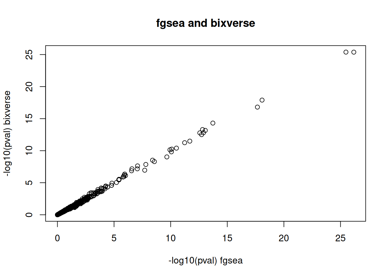
#> 6: 60406,20018,245688,20017 237 0.08175156The p-values from both implementations are in close agreement, as expected:
plot(
  x = -log10(fgsea_res$pval),
  y = -log10(bixverse_fgsea$pvals),
  xlab = "-log10(pval) fgsea",
  ylab = "-log10(pval) bixverse",
  main = "fgsea and bixverse"
)
The Rust implementation is consistently faster than fgsea’s Rcpp backend — not by an enormous margin on small data (roughly 20% in typical benchmarks), but the gap widens with the number of pathways and permutations:
microbenchmark::microbenchmark(
  fgsea = fgsea(
    pathways = examplePathways,
    stats = exampleRanks,
    minSize = 15,
    maxSize = 500
  ),
  rust = calc_fgsea(
    stats = exampleRanks,
    pathways = examplePathways,
    gsea_params = params_gsea(min_size = 15L)
  ),
  times = 5L
)
#> Unit: seconds
#>   expr     min       lq     mean   median       uq      max neval
#>  fgsea 2.40426 2.438197 2.613924 2.576308 2.679570 2.971285     5
#>   rust 2.16457 2.179880 2.195300 2.205283 2.208558 2.218208     5
GO-aware GSEA: the elimination method
bixverse combines the elimination method with GSEA, using the same GeneOntologyElim object as the hypergeometric variant. The ontology is traversed leaf-first; for each term a permutation-based p-value is computed and if it falls below the elimination threshold, genes from that term are removed from all ancestors before they are tested. Once the full traversal is complete, the fgsea multilevel method is applied to terms that reached nominal significance to obtain more precise p-values than pure permutation alone can provide.
gene_universe_go <- unique(
  unlist(go_data_dt[, "ensembl_id"], use.names = FALSE)
)

set.seed(42L)

random_stats <- rnorm(length(gene_universe_go))
names(random_stats) <- gene_universe_go

go_gsea_res <- fgsea_go_elim(
  object = go_data_s7,
  stats = random_stats
)

head(go_gsea_res)
#>         go_id         es       nes  size        pvals n_more_extreme
#>        <char>      <num>     <num> <num>        <num>          <num>
#> 1: GO:0031465 -0.9025468 -1.925965     6 6.165332e-05              0
#> 2: GO:0050877  0.5116421  1.950886    44 2.410338e-04              2
#> 3: GO:0072675 -0.8744037 -1.865910     6 2.625170e-04              0
#> 4: GO:0006066 -0.6718553 -2.026201    18 2.712234e-04              0
#> 5: GO:0071392 -0.5217830 -1.904151    36 3.788231e-04              0
#> 6: GO:0002090 -0.8302363 -1.868975     7 6.827804e-04              3
#>                                                                                               leading_edge
#>                                                                                                     <list>
#> 1:                                                         ENSG00000110844,ENSG00000180370,ENSG00000160685
#> 2: ENSG00000131263,ENSG00000229674,ENSG00000172987,ENSG00000108878,ENSG00000050165,ENSG00000143061,...[19]
#> 3:                                                                                         ENSG00000170613
#> 4:  ENSG00000287395,ENSG00000139354,ENSG00000211659,ENSG00000160345,ENSG00000007237,ENSG00000139679,...[7]
#> 5: ENSG00000118193,ENSG00000134531,ENSG00000166897,ENSG00000162980,ENSG00000170348,ENSG00000103018,...[17]
#> 6:                                         ENSG00000061938,ENSG00000169507,ENSG00000289721,ENSG00000083814
#>      log2err       fdr                                 go_name
#>        <num>     <num>                                  <char>
#> 1: 0.5384341 0.4815124  Cul4B-RING E3 ubiquitin ligase complex
#> 2: 0.5188481 0.5295637                  nervous system process
#> 3: 0.4984931 0.5295637                       osteoclast fusion
#> 4: 0.4984931 0.5295637               alcohol metabolic process
#> 5: 0.4984931 0.5917217 cellular response to estradiol stimulus
#> 6: 0.4772708 0.8290480  regulation of receptor internalization