
library(manifoldsR)
library(magrittr)
library(ggplot2)
library(data.table)
#>
#> Attaching package: 'data.table'
#> The following object is masked from 'package:base':
#>
#> %notin%DREAMS in manifoldsR
The t-SNE vignette has a warning in it: distances between clusters mean nothing. Two blobs sitting next to each other might be miles apart in the input space. PCA has the opposite problem. The global layout is faithful, but everything local gets squashed into an overlapping mess.
DREAMS sits in between. It is t-SNE with an extra pull towards a global reference embedding, PCA by default. You keep the clusters of t-SNE and their positions relative to each other start meaning something again. Original work by Kury, Kobak & Damrich, Transactions on Machine Learning Research, 2026.
Intro
Every t-SNE epoch, DREAMS scales the usual update by 1 - lambda and adds a quadratic pull towards the reference:
is the centred reference, rescales it to the current size of the embedding, and is the automatic openTSNE learning rate. The optimisation starts from the reference too, so the init element of params_tsne() is ignored.
One knob, set via params_dreams():
-
lambda. Regularisation strength in[0, 1].0is t-SNE (started from the reference),1returns the reference. Defaults to0.15, the value from the paper.
The regulariser is O(n) per epoch on top of the Barnes-Hut or FFT repulsion, so DREAMS costs about what t-SNE costs. Every approx_type from tsne() works here as well.
Measuring both ends
We need two numbers per embedding. Global: the Spearman correlation between subcluster centroid distances in the input and in the embedding. Local: the fraction of each point’s 15 nearest neighbours that survive the embedding.
global_preservation <- function(data, embd, membership) {
  centroids <- function(x) {
    split(seq_len(nrow(x)), membership) %>%
      lapply(\(i) colMeans(x[i, , drop = FALSE])) %>%
      do.call(rbind, .)
  }
  cor(
    as.vector(dist(centroids(data))),
    as.vector(dist(centroids(embd))),
    method = "spearman"
  )
}

knn_preservation <- function(data, embd, k = 15L) {
  idx <- function(x) {
    generate_knn_graph(
      data = x,
      k = k,
      knn_method = "exhaustive",
      .verbose = FALSE
    ) %>%
      get_idx_mat()
  }
  idx_data <- idx(data)
  idx_embd <- idx(embd)
  mean(vapply(
    seq_len(nrow(idx_data)),
    \(i) length(intersect(idx_data[i, ], idx_embd[i, ])) / k,
    numeric(1)
  ))
}
The hierarchical generator gives us 16 subclusters, grouped into 4 supergroups, in 50 dimensions. Subclusters within a supergroup are close, supergroups are far apart. Exactly the structure t-SNE throws away.
hierarchical_data <- manifold_synthetic_data(
  type = "hierarchical",
  n_samples = 5000L,
  dim = 50L,
  parameters = params_hierarchical(n_supergroups = 4L, n_subclusts = 4L)
)

subgroup <- hierarchical_data$membership$subgroup
supergroup <- hierarchical_data$membership$supergroup
PCA vs t-SNE vs DREAMS
embeddings <- list(PCA = pca_res, tSNE = tsne_res, DREAMS = dreams_res)

plot_df <- lapply(embeddings, \(embd) {
  data.table(
    dim1 = embd[, 1],
    dim2 = embd[, 2],
    supergroup = as.factor(supergroup),
    subgroup = as.factor(subgroup)
  )
}) %>%
  rbindlist(idcol = "method") %>%
  .[, method := factor(method, levels = names(embeddings))]

ggplot(
  data = plot_df,
  mapping = aes(x = dim1, y = dim2)
) +
  geom_point(
    mapping = aes(colour = supergroup, shape = subgroup),
    alpha = 0.5,
    size = 0.75
  ) +
  scale_shape_manual(values = rep(c(16, 17, 15, 3), 4), guide = "none") +
  facet_wrap(~method, scales = "free") +
  theme_bw() +
  xlab("Dim 1") +
  ylab("Dim 2") +
  ggtitle("Hierarchical data, coloured by supergroup")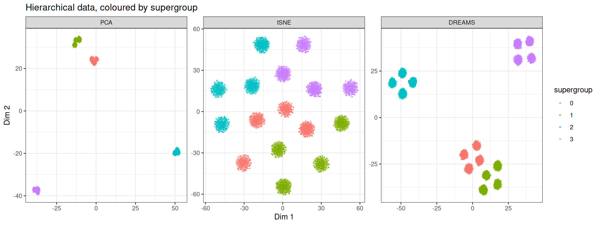
PCA gets the four supergroups in the right places and smears the subclusters within them. t-SNE separates all 16 subclusters cleanly, and then scatters them over the plane with no regard for which supergroup they belong to. DREAMS keeps the 16 subclusters separated and keeps each supergroup together.
lapply(embeddings, \(embd) {
  data.table(
    global = global_preservation(hierarchical_data$data, embd, subgroup),
    local = knn_preservation(hierarchical_data$data, embd)
  )
}) %>%
  rbindlist(idcol = "method") %>%
  .[, lapply(.SD, round, 3), by = method]
#>    method global local
#>    <char>  <num> <num>
#> 1:    PCA  0.896 0.061
#> 2:   tSNE  0.514 0.241
#> 3: DREAMS  0.891 0.211
The numbers say the same thing. DREAMS matches PCA on the global score and keeps most of the kNN preservation of t-SNE. PCA’s local score is dismal: two dimensions out of fifty is not enough to keep anyone’s neighbours.
Tuning lambda
lambda trades one end against the other. A sweep from t-SNE to PCA:
lambdas <- c(0, 0.05, 0.15, 0.5, 1)

lambda_sweep <- lapply(lambdas, \(lambda) {
  dreams(
    data = hierarchical_data$data,
    dreams_params = params_dreams(lambda = lambda),
    seed = 42L,
    .verbose = FALSE
  )
})
names(lambda_sweep) <- sprintf("lambda = %.2f", lambdas)

lapply(lambda_sweep, \(embd) {
  data.table(
    global = global_preservation(hierarchical_data$data, embd, subgroup),
    local = knn_preservation(hierarchical_data$data, embd)
  )
}) %>%
  rbindlist(idcol = "lambda") %>%
  .[, lapply(.SD, round, 3), by = lambda]
#>           lambda global local
#>           <char>  <num> <num>
#> 1: lambda = 0.00  0.438 0.240
#> 2: lambda = 0.05  0.798 0.239
#> 3: lambda = 0.15  0.891 0.211
#> 4: lambda = 0.50  0.912 0.144
#> 5: lambda = 1.00  0.896 0.061
sweep_df <- lapply(lambda_sweep, \(embd) {
  data.table(
    dim1 = embd[, 1],
    dim2 = embd[, 2],
    supergroup = as.factor(supergroup)
  )
}) %>%
  rbindlist(idcol = "lambda") %>%
  .[, lambda := factor(lambda, levels = names(lambda_sweep))]

ggplot(
  data = sweep_df,
  mapping = aes(x = dim1, y = dim2)
) +
  geom_point(mapping = aes(colour = supergroup), alpha = 0.5, size = 0.5) +
  facet_wrap(~lambda, scales = "free", ncol = 3) +
  theme_bw() +
  xlab("Dim 1") +
  ylab("Dim 2") +
  ggtitle("DREAMS lambda sweep")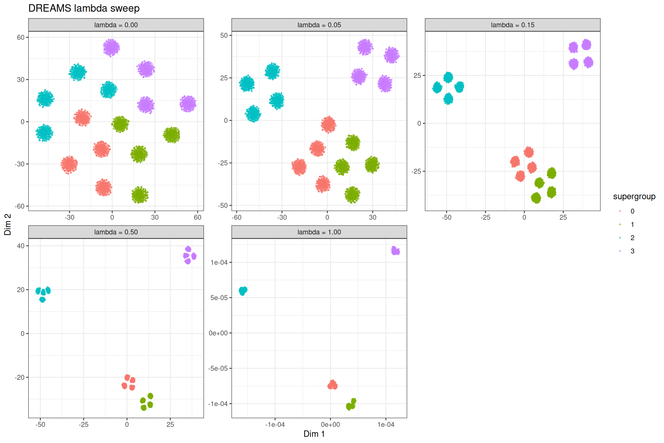
Even 0.05 buys most of the global structure back. The local score holds up to the default and then drops off fast. Past 0.5 you are looking at a slightly sharpened PCA. At 1 nothing moves at all: you get the reference at its initialisation scale (note the 1e-04 axes). The default is a sensible place to start; go lower if the subclusters start to touch.
Bring your own reference
PCA is a fine reference when the global structure is linear-ish. When it is not, hand DREAMS something better via reference: any samples x 2 matrix works, e.g. a PHATE or MDS embedding. On branching trajectory data PHATE is the obvious pick.
trajectory_data <- manifold_synthetic_data(
  type = "trajectory",
  n_samples = 5000L
)

phate_traj <- phate(
  data = trajectory_data$data,
  k = 15L,
  seed = 42L,
  .verbose = TRUE
)

tsne_traj <- tsne(
  data = trajectory_data$data,
  seed = 42L,
  .verbose = TRUE
)

dreams_traj <- dreams(
  data = trajectory_data$data,
  reference = phate_traj,
  seed = 42L,
  .verbose = TRUE
)
traj_embeddings <- list(
  PHATE = phate_traj,
  tSNE = tsne_traj,
  `DREAMS (PHATE reference)` = dreams_traj
)

traj_df <- lapply(traj_embeddings, \(embd) {
  data.table(
    dim1 = embd[, 1],
    dim2 = embd[, 2],
    branch = as.factor(trajectory_data$membership)
  )
}) %>%
  rbindlist(idcol = "method") %>%
  .[, method := factor(method, levels = names(traj_embeddings))]

ggplot(
  data = traj_df,
  mapping = aes(x = dim1, y = dim2)
) +
  geom_point(mapping = aes(colour = branch), alpha = 0.5, size = 0.5) +
  facet_wrap(~method, scales = "free") +
  theme_bw() +
  xlab("Dim 1") +
  ylab("Dim 2") +
  ggtitle("Trajectory data, coloured by branch")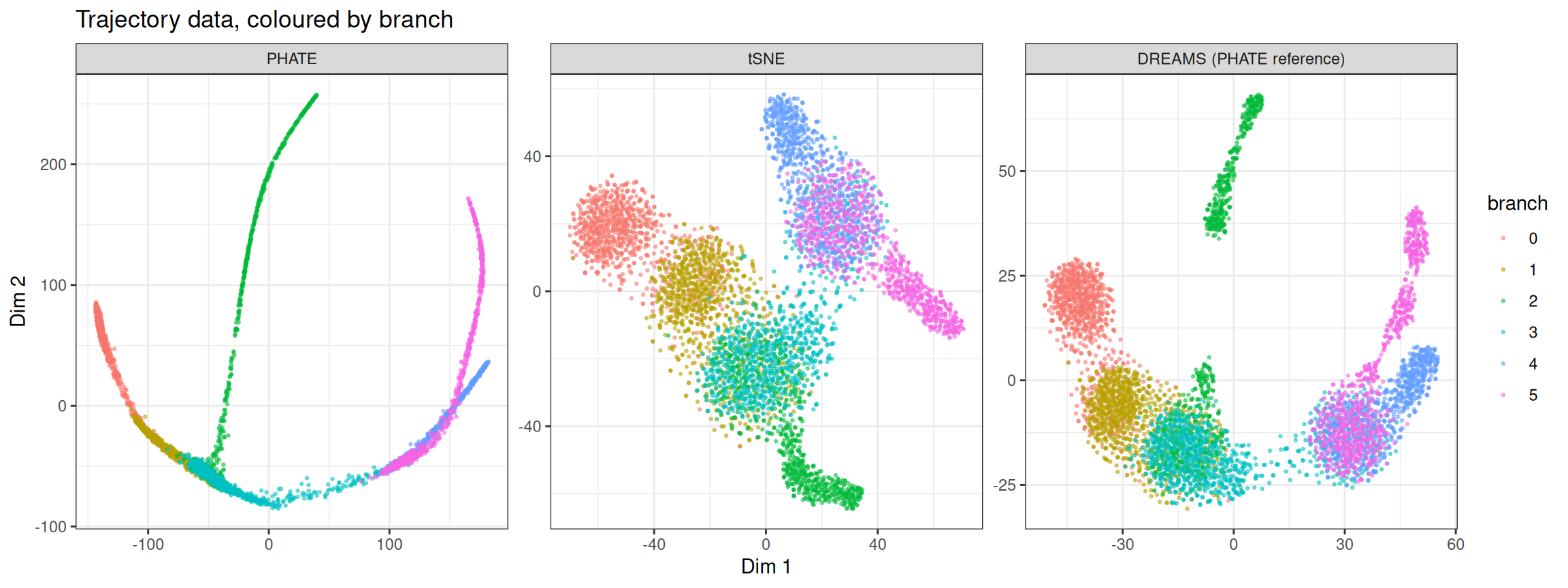
Mixed bag. The branch order along the main stem follows PHATE, where t-SNE just piles branches 3 and 5 on top of each other. But the long PHATE tips of branches 2 and 5 tear off into separate islands. That’s DREAMS itself, not this implementation: the authors’ openTSNE fork breaks the same two branches into the same number of pieces on this data, with a PCA reference as well. At lambda = 0.05 both branches stay in one piece, so on long trajectories go lower than the default.
Already have a NearestNeighbours object? Pass it via knn = and DREAMS skips the search, same as every other method in the package.