library(bixverse)
library(bixverse.plots)
library(data.table)
#>
#> Attaching package: 'data.table'
#> The following object is masked from 'package:base':
#>
#>     %notin%
library(ggplot2)
library(magrittr)
Clustering, cell type annotation and reference mapping
2026-10-27
Intro
Getting from a corrected embedding to cell type labels involves more choices than a single find_clusters_sc() call suggests. Which graph do you cluster on? Leiden or Louvain, and how many iterations? Do you cluster every cell, or coarsen first because you have a million of them? Do you stamp one label per cluster, or score each cell? And once you have a well annotated data set, how do you avoid redoing all of it every time a new sample lands on your desk?
This vignette goes through these decisions in that order:
- Build a reference from two PBMC data sets (pbmc3k + pbmc4k), corrected with Harmony v2.
- Compare the three neighbour graphs bixverse can build (sNN, the UMAP fuzzy simplicial set and the plain kNN union) and what they do to the clustering.
- Leiden vs Louvain, and the fast clustering via k-means coarsening.
- Annotate with scType, per cluster and per cell.
- Compress the reference with Symphony (Kang, et al., 2021), map a third PBMC data set (pbmc8k) into it and transfer the labels.
If you have not read the batch correction vignette and the introductory vignette, please do so first; this vignette assumes familiarity with both.
Building the reference data
Loading the reference batches
We use the same pbmc3k + pbmc4k pair as in the batch correction vignette. Two batches with the same broad cell type composition and a clear technical difference between them is exactly the situation Symphony is designed for: the reference learns the batch correction once, and that correction can then be applied to future queries without rerunning Harmony.
Code
dir_data <- download_pbmc_batches()

tempdir_ref <- file.path(tempdir(), "symphony_ref")
dir.create(tempdir_ref, showWarnings = FALSE, recursive = TRUE)

h5ad_files <- list.files(dir_data)
h5ad_files <- h5ad_files[grepl(".h5ad", h5ad_files)]
h5ad_paths <- file.path(dir_data, h5ad_files)
names(h5ad_paths) <- c("pbmc3k", "pbmc4k")

h5_tasks <- prescan_h5ad_files(h5_paths = h5ad_paths)

sc_ref <- SingleCells(dir_data = tempdir_ref)

sc_ref <- load_multi_h5ad(
  object = sc_ref,
  prescan_result = h5_tasks,
  .verbose = TRUE
)
#>  Converting the cell-based data into the gene-based format.
#> Loading observation data from h5ad files into DuckDB.
#> Loading variable data into DuckDB.
Quality control
Standard QC: mitochondrial gene proportions, library complexity, MAD-based outlier detection.
Code
var_ref <- get_sc_var(sc_ref)

# let's get the gene symbols from one of the h5ad files - in multi file import
# additional columns are dropped from the vars
h5_metadata <- read_h5ad_metadata(h5ad_paths[[1]])

var_ref <- merge(
  var_ref,
  h5_metadata$var[, c("ENSEMBL_ID", "Symbol_TENx")],
  by.x = "gene_id",
  by.y = "ENSEMBL_ID"
)

setnames(var_ref, old = "Symbol_TENx", new = "gene_symbol", skip_absent = TRUE)

gs_of_interest <- list(
  MT = var_ref[grepl("^MT-", gene_symbol), gene_id],
  Ribo = var_ref[grepl("^RPS|^RPL", gene_symbol), gene_id]
)

sc_ref <- gene_set_proportions_sc(
  sc_ref,
  gs_of_interest,
  streaming = FALSE,
  .verbose = TRUE
)

qc_df <- sc_ref[[c("cell_id", "lib_size", "nnz", "MT", "exp_id")]]

metrics <- list(
  log10_lib_size = log10(qc_df$lib_size),
  log10_nnz = log10(qc_df$nnz),
  MT = qc_df$MT
)
directions <- c(
  log10_lib_size = "twosided",
  log10_nnz = "twosided",
  MT = "above"
)

qc <- run_cell_qc(
  metrics = metrics,
  cells_to_keep = get_cells_to_keep(sc_ref),
  directions = directions,
  threshold = 3
)

sc_ref[["outlier"]] <- qc$combined
cells_to_keep <- qc_df[!qc$combined, cell_id]
sc_ref <- set_cells_to_keep(sc_ref, cells_to_keep)
HVGs, PCA, Harmony v2
This block is the Harmony v2 path of the batch correction vignette: pick HVGs, run PCA, run Harmony v2. Version 1 is still available via harmony_sc() and params_sc_harmony(), but v2 is preferable in most settings (see the batch correction vignette for the reasoning).
sc_ref <- find_hvg_sc(
  object = sc_ref,
  hvg_no = 2000L,
  .verbose = TRUE
)

sc_ref <- calculate_pca_sc(
  object = sc_ref,
  no_pcs = 30L
)
#> Using sparse SVD solving on scaled data on 2000 HVG.

sc_ref <- harmony_v2_sc(
  object = sc_ref,
  batch_column = "exp_id",
  harmony_params = params_sc_harmony_v2()
)
#>  Auto-determined number of Harmony clusters: 100
Which graph to cluster on
find_neighbours_sc() does two things: it finds the kNN on the embedding and it symmetrises that kNN into the undirected, weighted graph the clustering runs on. The second step is controlled by knn_sym in params_knn_graph_defaults(), passed via graph in params_sc_neighbours(). Three options:
-
"snn"(default): the shared nearest neighbour graph of bluster/Seurat. Two cells are linked if their neighbourhoods overlap, weighted by Jaccard (or rank), and weak edges belowpruningare dropped. -
"umap": the fuzzy simplicial set from UMAP, i.e. what ScanPy stores inobsp/connectivities. Use this if you want your Leiden clusters to line up with a ScanPy pipeline. -
"knn": the plain union of the kNN, every edge weighted 1.
Let’s build all three on the Harmony embedding and cluster each across a few resolutions. Every call recomputes the kNN as well, which at ~7k cells costs nothing.
graph_types <- c("snn", "umap", "knn")
resolutions <- c(0.5, 1, 1.5, 2)

n_clusters <- purrr::map(graph_types, \(graph_type) {
  sc_ref <- find_neighbours_sc(
    object = sc_ref,
    embd_to_use = "harmony_v2",
    neighbours_params = params_sc_neighbours(
      graph = list(knn_sym = graph_type)
    ),
    .verbose = FALSE
  )

  purrr::map(resolutions, \(res) {
    col_name <- sprintf("leiden_%s_%s", graph_type, res)
    sc_ref <- find_clusters_sc(sc_ref, res = res, name = col_name)
    data.table(
      graph = graph_type,
      resolution = res,
      n_clusters = uniqueN(unlist(sc_ref[[col_name]]))
    )
  }) %>%
    rbindlist()
}) %>%
  rbindlist()

dcast(n_clusters, resolution ~ graph, value.var = "n_clusters")
#> Key: <resolution>
#>    resolution   knn   snn  umap
#>         <num> <int> <int> <int>
#> 1:        0.5    10    13    11
#> 2:        1.0    12    15    16
#> 3:        1.5    17    20    22
#> 4:        2.0    23    22    26
The point of this table: resolutions do not carry over between graphs. The "umap" and "knn" graphs only hold the kNN pairs, while the sNN graph also links cells that merely share neighbours and prunes weak edges. On this data the differences are a handful of communities at a given resolution, and not always in the same direction. On other data they can be larger. If you move a ScanPy pipeline over and switch to knn_sym = "umap", keep its resolution; if you switch to sNN, retune it.
For the rest of the vignette we work on the sNN graph.
sc_ref <- find_neighbours_sc(
  object = sc_ref,
  embd_to_use = "harmony_v2",
  neighbours_params = params_sc_neighbours()
)
#>
#> Generating the snn graph.

sc_ref <- umap_sc(
  sc_ref,
  slot_name = "umap_harm_v2",
  use_knn = TRUE
)
#> Running UMAP.
#> Using n_epochs = 500 (dataset <10k samples or adam_parallel optimiser)
#> Using provided kNN graph.
Clustering
Leiden vs Louvain
Both run in Rust, and the labels depend on seed only, not on the global RNG or the number of threads. Leiden is the default; it guarantees connected communities, which Louvain does not (Traag, et al., 2019). Labels are 0-based with 0 being the largest cluster.
sc_ref <- find_clusters_sc(sc_ref, res = 1, name = "leiden_clusters")

sc_ref <- find_clusters_sc(
  sc_ref,
  cluster_algorithm = "louvain",
  res = 1,
  name = "louvain_clusters"
)
A few knobs get passed through ... to leiden_clustering():
-
n_iterations: defaults to2Lfor Louvain and5Lfor Leiden. A negative value iterates until the partition is stable. -
min_gain: with a negativen_iterations, also stop once an iteration gains no more than this in modularity. -
local_moving:"queue"is Traag’s sequential queue,"coloured"moves the nodes of one colour class in parallel. The latter only kicks in on the larger levels of the graph, so on 7k cells don’t expect much.
sc_ref <- find_clusters_sc(
  sc_ref,
  res = 1,
  name = "leiden_stable",
  n_iterations = -1L,
  min_gain = 1e-4,
  local_moving = "coloured"
)
How much do the three labelings agree? A small helper that plots, for each cluster of one labeling, how its cells spread across the clusters of another:
plot_overlap <- function(a, b, name_a, name_b) {
  dt <- data.table(a = factor(a), b = factor(b))[, .N, by = .(a, b)] %>%
    .[, frac := N / sum(N), by = a]

  # light text on the dark end of viridis, dark text on the yellow end
  ggplot(dt, aes(x = b, y = a, fill = frac)) +
    geom_tile() +
    geom_text(
      aes(
        label = sprintf("%.2f", frac),
        colour = ifelse(frac < 0.5, "white", "black")
      ),
      size = 2.5
    ) +
    scale_colour_identity() +
    scale_fill_viridis_c(limits = c(0, 1)) +
    labs(x = name_b, y = name_a, fill = "Fraction:") +
    theme_minimal()
}
clusters_dt <- sc_ref[[c(
  "leiden_clusters",
  "louvain_clusters",
  "leiden_stable"
)]]

plot_overlap(
  clusters_dt$leiden_clusters,
  clusters_dt$louvain_clusters,
  "Leiden",
  "Louvain"
) +
  ggtitle("Leiden vs Louvain (res = 1)")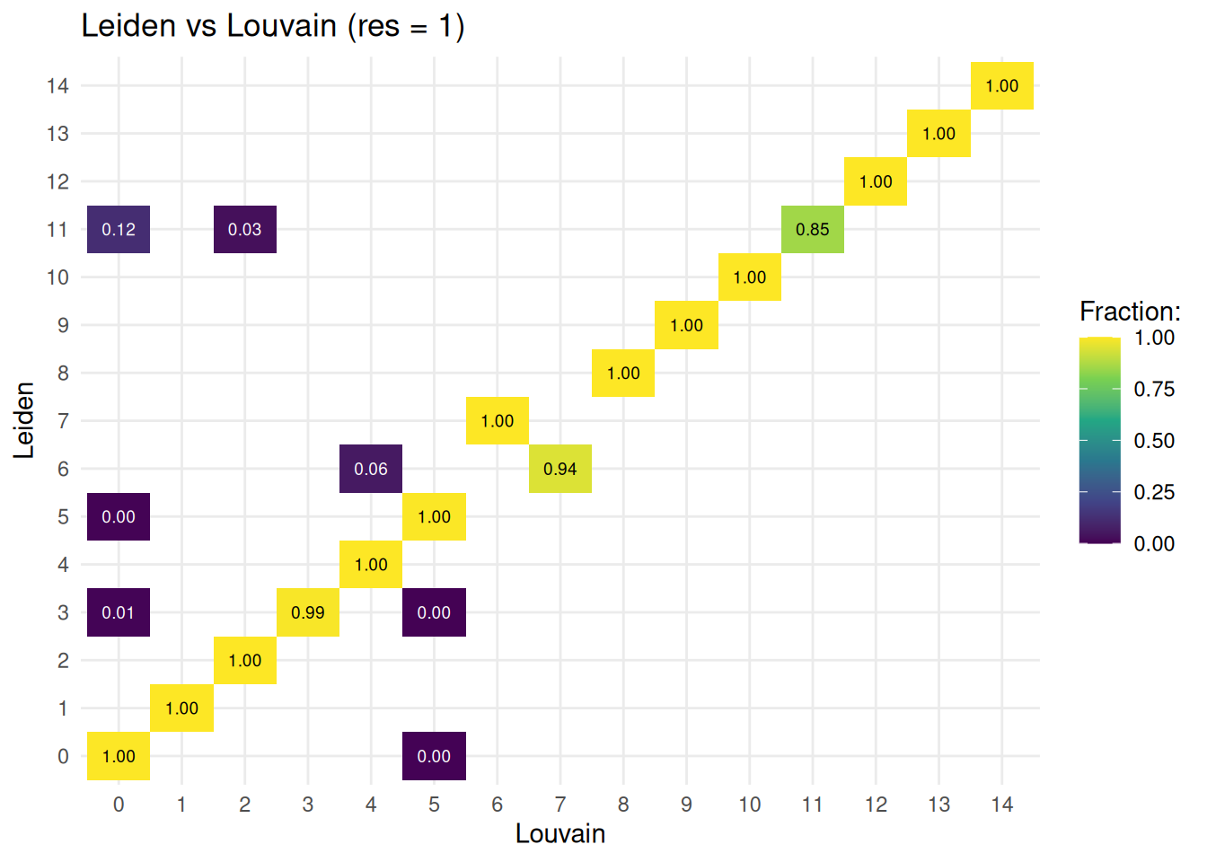
plot_overlap(
  clusters_dt$leiden_clusters,
  clusters_dt$leiden_stable,
  "Leiden (5 iterations)",
  "Leiden (until stable)"
) +
  ggtitle("Fixed iterations vs iterating until stable")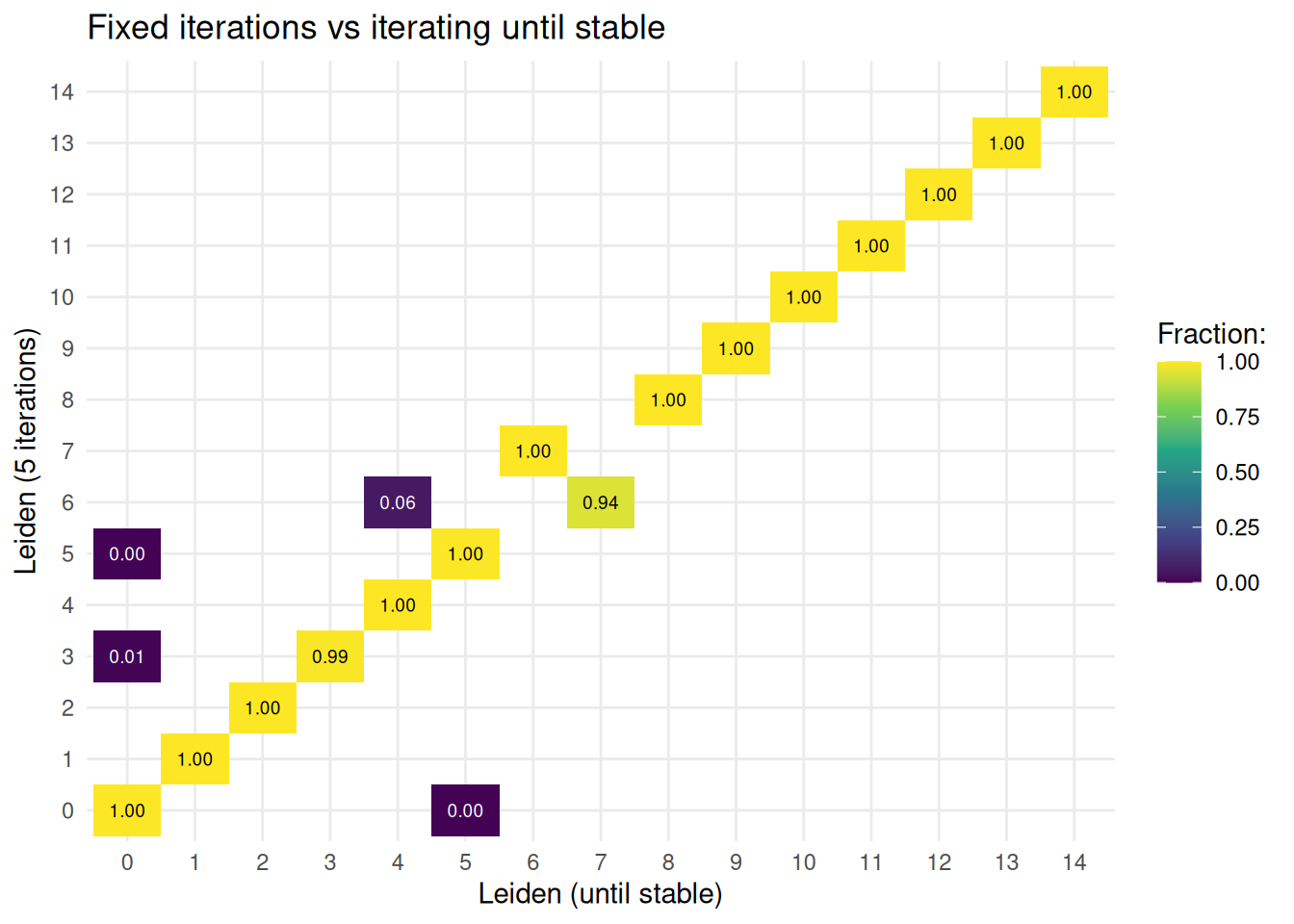
Fast clustering
On a few thousand cells the full graph clustering is instant. On a million it isn’t. fast_cluster_sc() coarsens the cells with k-means first (sqrt(N) centroids by default), builds a graph over the centroids and runs Louvain or Leiden on that. Each cell inherits the community of its centroid. Two options for the centroid graph:
- the default, a symmetrised kNN between the centroids (
centroid_k,centroid_graph); -
cell_mediated = TRUE, the Secuer graph (Wei, et al., PLoS Comput Biol, 2022), where each cell links itsn_anchorsnearest centroids, so two centroids are connected if they share cells.
With n_seeds > 1 every resolution is run once per seed. The labels of the seed with the lowest mean conductance are kept, and the ARI and conductance across seeds come back as stability statistics.
fc_resolutions <- c(2, 1.5, 1, 0.5)

fc_knn <- fast_cluster_sc(
  object = sc_ref,
  embd_to_use = "harmony_v2",
  resolutions = fc_resolutions,
  n_seeds = 10L
)

fc_cell_med <- fast_cluster_sc(
  object = sc_ref,
  embd_to_use = "harmony_v2",
  resolutions = fc_resolutions,
  fc_params = params_sc_fast_cluster(cell_mediated = TRUE),
  n_seeds = 10L
)
The stats help to pick a resolution: high ARI means the partition barely changes between seeds, low conductance means the communities are well separated in the centroid graph.
fc_stats <- rbindlist(list(
  fc_knn$stats[, graph := "centroid kNN"],
  fc_cell_med$stats[, graph := "cell-mediated"]
))

fc_stats
#>    resolution  mean_ari median_ari mean_conductance median_conductance
#>         <num>     <num>      <num>            <num>              <num>
#> 1:        2.0 0.9828833  0.9823357       0.19748537         0.18767531
#> 2:        1.5 1.0000000  1.0000000       0.05310797         0.06072441
#> 3:        1.0 1.0000000  1.0000000       0.05228200         0.05938450
#> 4:        0.5 1.0000000  1.0000000       0.05178834         0.05776583
#> 5:        2.0 0.9464080  0.9424633       0.23830207         0.18086970
#> 6:        1.5 0.9378425  0.9501527       0.18763205         0.14751919
#> 7:        1.0 0.9744326  0.9712801       0.11759994         0.12176237
#> 8:        0.5 0.9500480  0.9645567       0.08086254         0.07918369
#>    mean_n_comms         graph
#>           <num>        <char>
#> 1:          8.0  centroid kNN
#> 2:          5.0  centroid kNN
#> 3:          5.0  centroid kNN
#> 4:          5.0  centroid kNN
#> 5:         14.6 cell-mediated
#> 6:         12.6 cell-mediated
#> 7:          9.0 cell-mediated
#> 8:          6.8 cell-mediated

melt(
  fc_stats,
  id.vars = c("graph", "resolution"),
  measure.vars = c("mean_ari", "mean_conductance")
) %>%
  ggplot(aes(x = resolution, y = value, colour = graph)) +
  geom_line() +
  geom_point() +
  facet_wrap(~variable, scales = "free_y") +
  labs(x = "Resolution", y = NULL, colour = "Centroid graph:") +
  theme_minimal()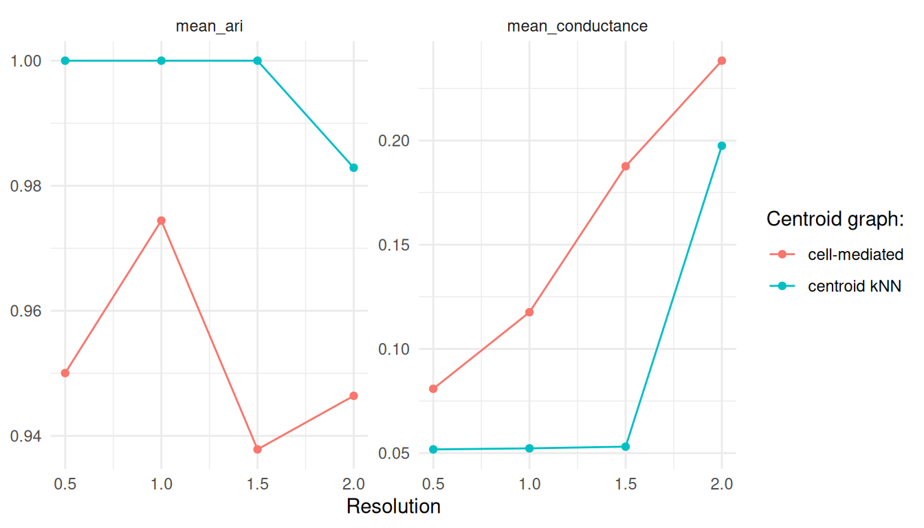
And how does the coarsened version compare against Leiden on the full graph?
sc_ref <- add_sc_new_obs(
  object = sc_ref,
  obs_data = get_data(fc_cell_med)
)

fast_dt <- sc_ref[[c("leiden_clusters", "res_1")]]

plot_overlap(
  fast_dt$leiden_clusters,
  fast_dt$res_1,
  "Leiden (full graph)",
  "Fast clustering (cell-mediated, res = 1)"
) +
  ggtitle("Full vs fast clustering")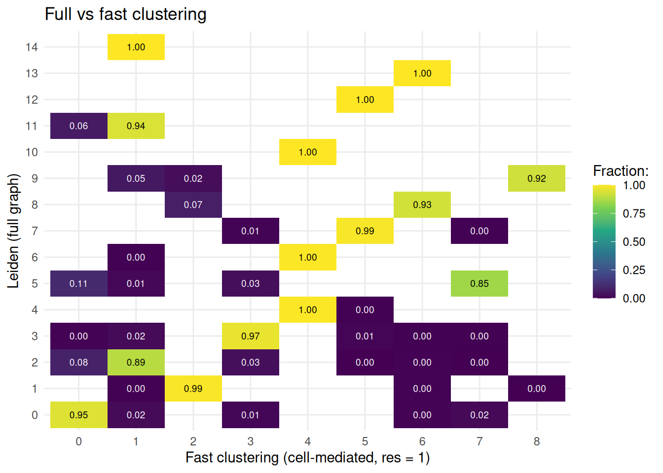
With ~5.8k cells there are only ~76 centroids, so the partitions come out coarse: about 5 communities at resolution 1 against 14 for Leiden on the full graph. For data sets of this size, stick with find_clusters_sc(). The fast path earns its keep once you are in the hundreds of thousands of cells, see the 1 million cells vignette.
Cell type annotation
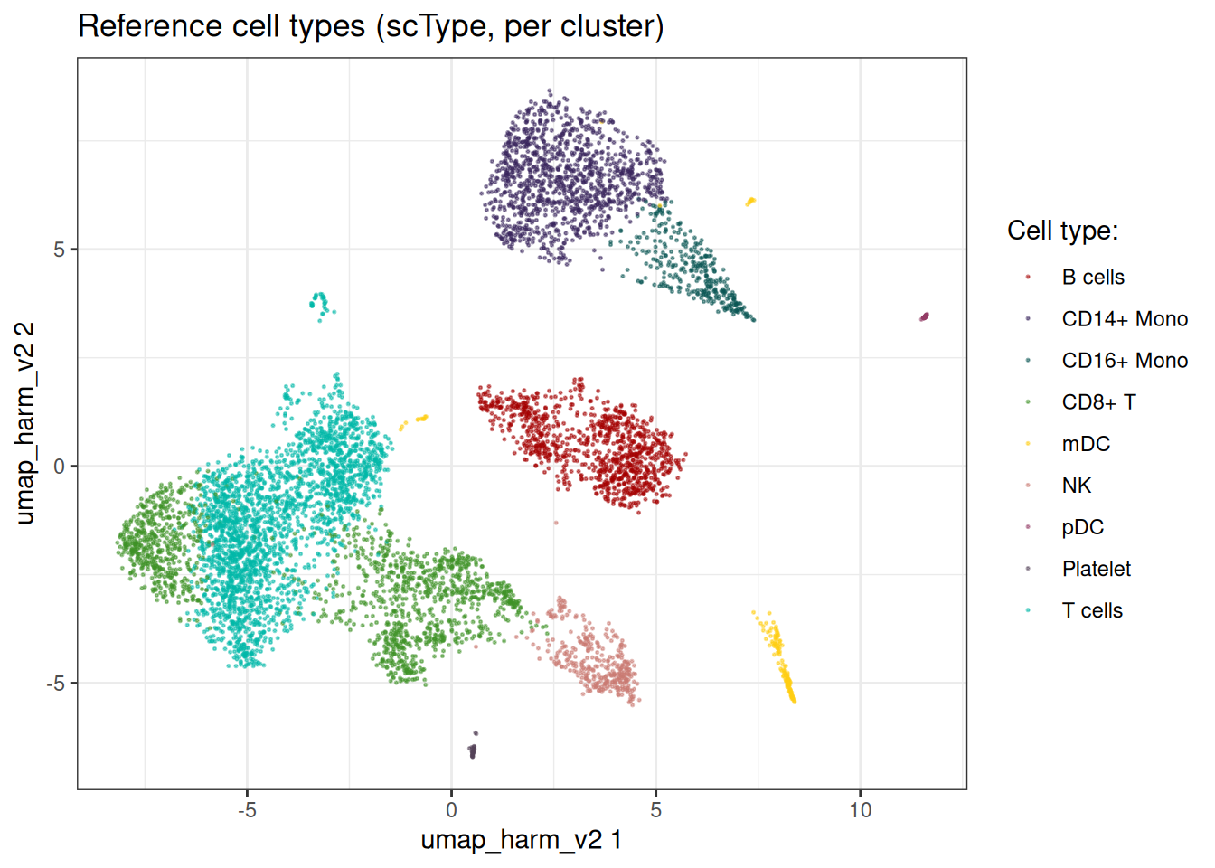
scType per cluster
We annotate with scType (Ianevski, et al., Nat Comm, 2022) using a PBMC marker set.
cell_markers <- c(
  CD3D = "T cells",
  CD3E = "T cells",
  CD3G = "T cells",
  IL7R = "CD4+ T",
  CD4 = "CD4+ T",
  CD8A = "CD8+ T",
  CD8B = "CD8+ T",
  MS4A1 = "B cells",
  CD79A = "B cells",
  CD19 = "B cells",
  CD14 = "CD14+ Mono",
  LYZ = "CD14+ Mono",
  S100A8 = "CD14+ Mono",
  FCGR3A = "CD16+ Mono",
  CDKN1C = "CD16+ Mono",
  GNLY = "NK",
  NKG7 = "NK",
  NCAM1 = "NK",
  FCER1A = "mDC",
  CD1C = "mDC",
  LILRA4 = "pDC",
  CLEC4C = "pDC",
  PPBP = "Platelet",
  PF4 = "Platelet"
)
calc_sc_type_scores() scores every cell against every marker set, score_clusters() sums the scores per cluster and assigns the winner.
cell_markers_dt <- stack(cell_markers) %>%
  as.data.table() %>%
  setnames(., c("values", "ind"), c("cell_type", "gene_symbol")) %>%
  .[, gene_symbol := as.character(gene_symbol)] %>%
  .[, gene_id := var_ref$gene_id[match(gene_symbol, var_ref$gene_symbol)]] %>%
  .[!is.na(gene_id), ]

marker_list <- prepare_cell_markers(sc_ref, cell_markers_dt)

sctype_scores <- calc_sc_type_scores(
  object = sc_ref,
  cell_marker_list = marker_list
)

cell_type_anno <- score_clusters(
  sctype_scores,
  sc_ref[[]][["leiden_clusters"]]
)

obs <- get_sc_obs(sc_ref, filtered = TRUE)[, .(
  cell_idx,
  leiden_clusters
)] %>%
  .[,
    sc_type := cell_type_anno$cell_type[match(
      leiden_clusters,
      cell_type_anno$cluster_id
    )]
  ]

sc_ref[["sc_type"]] <- obs$sc_type
scType per cell
The cluster level call stamps one label on every cell of a cluster. A small population that shares a Leiden community with a bigger one gets absorbed and nothing flags it. assign_sc_type() scores per cell instead: the score matrix is smoothed over the neighbour graph via label spreading (Zhou, et al., NIPS, 2004), then each cell takes its own argmax. Cells whose best score falls below score_floor come back as NA. Pass cluster_col and you also get the per-cluster composition and a hybrid call: clusters at or above purity_threshold keep the cluster level label, mixed clusters fall back to the per-cell calls.
sctype_cells <- assign_sc_type(
  object = sc_ref,
  sc_type_res = sctype_scores,
  cluster_col = "leiden_clusters",
  sctype_cell_params = params_sctype_cells()
)
#> Assigning cell types per cell (smoothing: TRUE).

sctype_cells
#> ScTypeCellResults: 6626 cells, 10 cell types
#>   Unknown cells:  70
#>   Smoothing used: TRUE
#>   Mixed clusters: 8 out of 15

sc_ref[[c("sc_type_cell", "sc_type_hybrid", "sc_type_margin")]] <- list(
  sc_type_cell = sctype_cells$assignments,
  sc_type_hybrid = sctype_cells$hybrid,
  sc_type_margin = sctype_cells$margins
)
The composition table is the place to look for clusters that hide more than one cell type:
sctype_cells$composition
#>     cluster_id n_cells n_unknown   dominant    purity     second
#>          <int>   <int>     <int>     <char>     <num>     <char>
#>  1:          0    1304        62    T cells 0.7285276     CD4+ T
#>  2:          1    1106         0 CD14+ Mono 0.9882459   Platelet
#>  3:          2     956         5    T cells 0.6359833     CD4+ T
#>  4:          3     873         2     CD8+ T 0.4226804         NK
#>  5:          4     592         0    B cells 0.9966216        pDC
#>  6:          5     540         0     CD8+ T 0.8629630    T cells
#>  7:          6     343         0    B cells 0.9504373        mDC
#>  8:          7     338         0         NK 0.9881657 CD16+ Mono
#>  9:          8     306         0 CD16+ Mono 0.9346405 CD14+ Mono
#> 10:          9     130         0        mDC 0.8692307 CD14+ Mono
#> 11:         10      40         0        pDC 1.0000000       <NA>
#> 12:         11      34         1    T cells 0.6176471     CD4+ T
#> 13:         12      28         0    T cells 0.5000000     CD8+ T
#> 14:         13      25         0   Platelet 1.0000000       <NA>
#> 15:         14      11         0        mDC 0.7272727     CD4+ T
#>     second_fraction    entropy cluster_mixed
#>               <num>      <num>        <lgcl>
#>  1:     0.143404901 0.96370196          TRUE
#>  2:     0.006329114 0.07924042         FALSE
#>  3:     0.308577418 0.90547264          TRUE
#>  4:     0.278350502 1.27517283          TRUE
#>  5:     0.003378378 0.02259685         FALSE
#>  6:     0.122222222 0.46605775          TRUE
#>  7:     0.037900876 0.23082455         FALSE
#>  8:     0.005917160 0.07657434         FALSE
#>  9:     0.058823530 0.26271373         FALSE
#> 10:     0.084615387 0.49354321          TRUE
#> 11:     0.000000000 0.00000000         FALSE
#> 12:     0.352941185 0.76889431          TRUE
#> 13:     0.214285716 1.31297684          TRUE
#> 14:     0.000000000 0.00000000         FALSE
#> 15:     0.272727281 0.58595264          TRUE
Most of the mixed clusters are T cell clusters split between "T cells" and "CD4+ T" or "CD8+ T". That is the marker set, not the method: the generic "T cells" set (CD3D/E/G) competes with the subtype sets on the same cells. A hierarchical marker set, or dropping the generic T cell entry, cleans this up.
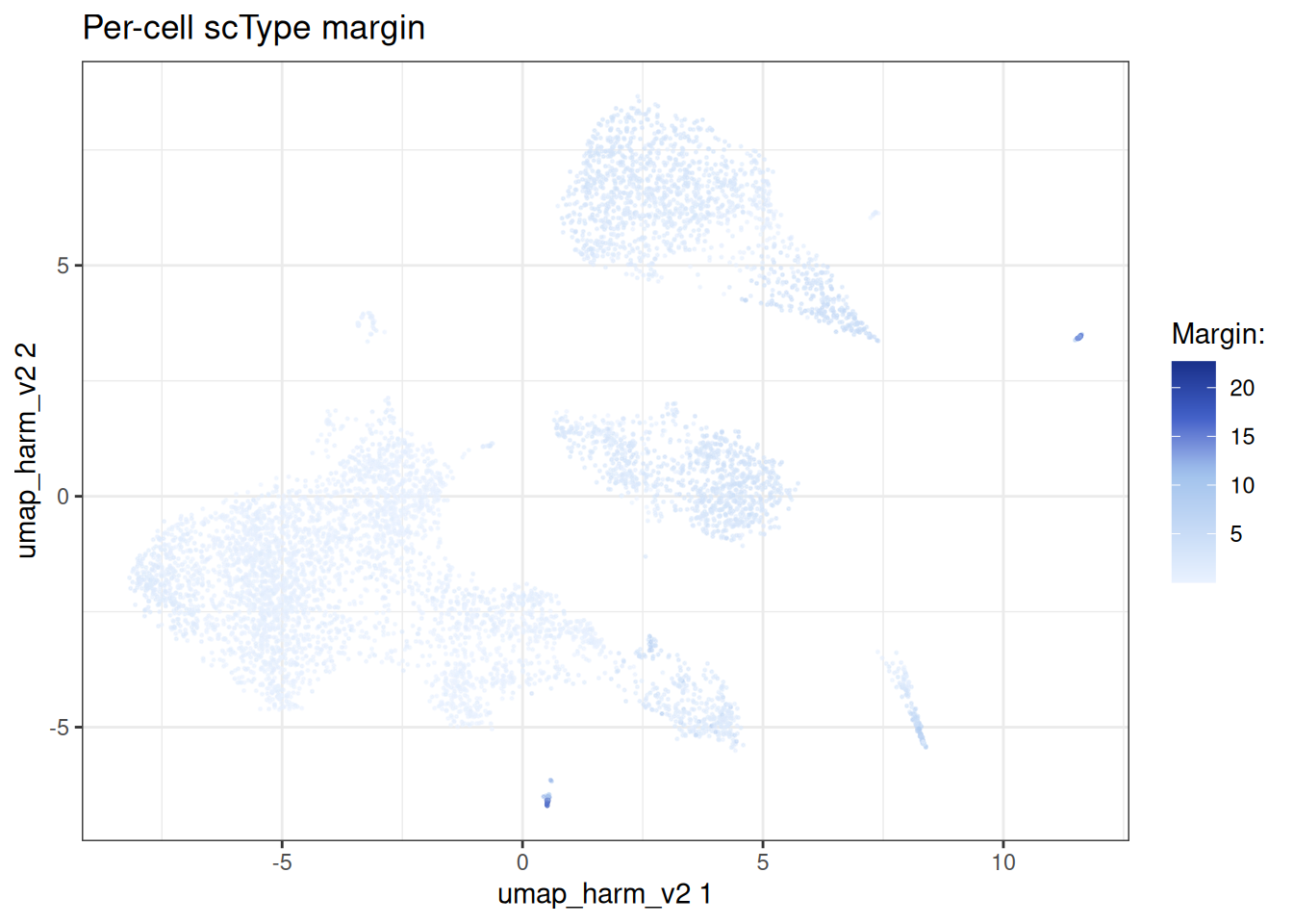
The margin (best minus second best score) flags ambiguous calls:
embedding_plot_sc(
  sc_ref,
  embedding = "umap_harm_v2",
  colour_by = "sc_type_margin",
  discrete = FALSE
) +
  labs(
    title = "Per-cell scType margin",
    colour = "Margin:"
  )
Sanity checks
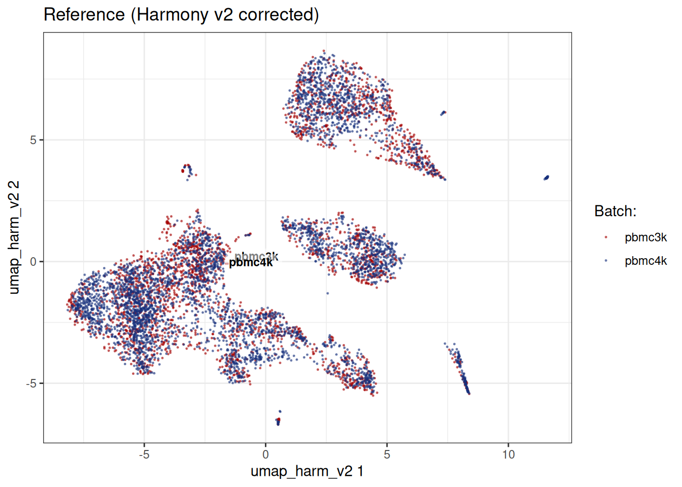
Batches mixed, cell types separated:
embedding_plot_sc(
  sc_ref,
  embedding = "umap_harm_v2",
  colour_by = "exp_id",
  label_by = "exp_id",
  discrete = TRUE
) +
  labs(
    title = "Reference (Harmony v2 corrected)",
    colour = "Batch:"
  )
embedding_plot_sc(
  sc_ref,
  embedding = "umap_harm_v2",
  colour_by = "sc_type",
  discrete = TRUE
) +
  labs(
    title = "Reference cell types (scType, per cluster)",
    colour = "Cell type:"
  )
embedding_plot_sc(
  sc_ref,
  embedding = "umap_harm_v2",
  colour_by = "sc_type_hybrid",
  discrete = TRUE
) +
  labs(
    title = "Reference cell types (scType, hybrid)",
    colour = "Cell type:"
  )
#> Warning: Removed 70 rows containing missing values or values outside the scale range
#> (`geom_point()`).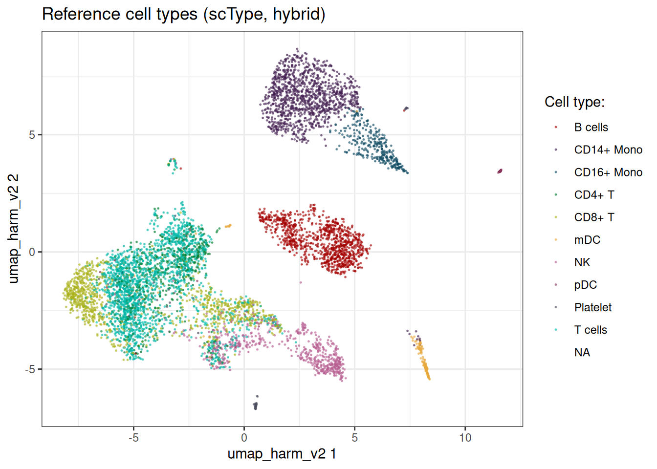
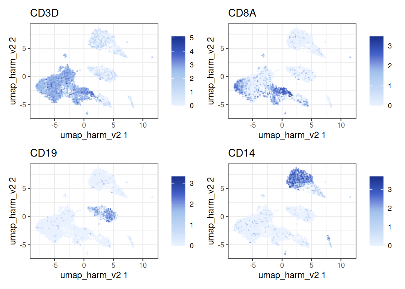
And the canonical markers:
feature_plot_sc(
  object = sc_ref,
  features = c(
    "ENSG00000167286",
    "ENSG00000153563",
    "ENSG00000177455",
    "ENSG00000170458"
  ),
  feature_labels = c(
    "ENSG00000167286" = "CD3D",
    "ENSG00000153563" = "CD8A",
    "ENSG00000177455" = "CD19",
    "ENSG00000170458" = "CD14"
  ),
  embedding = "umap_harm_v2"
)
Reference mapping with Symphony
Once you have a well annotated reference, you don’t want to redo QC, HVG selection, PCA, batch correction, clustering and manual annotation for every new sample. Symphony compresses the reference into a small set of cached terms that map new query cells into the same coordinate system in a single shot, with no need to keep the reference cells around at query time.
Compressing into a SymphonyReference
build_symphony_ref() re-runs PCA and Harmony internally using the supplied HVGs, then caches the loadings, centroids and compression terms (Nr, C) needed for query mapping. Pass label_columns to snapshot one or more obs columns, here both scType annotations, into the reference for downstream label transfer.
A note on the apparent duplication: yes, PCA + Harmony are run again inside build_symphony_ref(), even though we just ran them on the same HVGs above. This is deliberate. The standard pipeline keeps its embeddings on the SingleCells object and streams from disk; the Symphony reference keeps a self-contained, in-memory copy of everything it needs to project queries without the reference cells. Sharing state across those two representations would tie them together in unhelpful ways. The cost is one extra PCA + Harmony run at build time.
# needs +1L because 0-indexed HVGs are returned
hvg_indices <- get_hvg(sc_ref) + 1L

symphony_ref <- build_symphony_ref(
  object = sc_ref,
  batch_column = "exp_id",
  hvg = hvg_indices,
  harmony_params = params_sc_harmony_v2(),
  pca_params = params_sc_pca(),
  no_pcs = 30L,
  label_columns = c("sc_type", "sc_type_hybrid"),
  .verbose = TRUE
)
#>  Auto-determined number of Harmony clusters: 100

symphony_ref
#> Symphony reference
#>   Harmony backend: v2
#>   No HVGs: 2000
#>   No PCs: 30
#>   No clusters: 100
#>   Batch variables: exp_id
#>   Slim: FALSE
#>   Labels: sc_type, sc_type_hybrid
The print method tells you the Harmony backend, the size of the loadings and centroid matrices, the batch variables and the stored label columns.
Loading the query
We use pbmc8k as the query. Same tissue, same broad biology, but a different 10x run: exactly the kind of “another sample arrives” scenario Symphony is built for.
Code
pbmc8k_path <- download_pbmc8k()

tempdir_query <- file.path(tempdir(), "symphony_query")
dir.create(tempdir_query, showWarnings = FALSE, recursive = TRUE)

mtx_io_params <- get_cell_ranger_params(pbmc8k_path)

sc_query <- SingleCells(dir_data = tempdir_query)

sc_query <- load_mtx(
  object = sc_query,
  sc_mtx_io_param = mtx_io_params,
  mtx_streaming = FALSE,
  .verbose = TRUE
)
#>  Converting the cell-based data into the gene-based format.
#> Loading observations data from flat file into the DuckDB.
#> Loading variable data from flat file into the DuckDB.
Quality control on the query
Same QC as the reference. We are not trying to match library sizes or anything fancy across data sets, just remove clearly bad cells.
Code
var_q <- get_sc_var(sc_query)

gs_q <- list(
  MT = var_q[grepl("^MT-", column1), gene_id],
  Ribo = var_q[grepl("^RPS|^RPL", column1), gene_id]
)

sc_query <- gene_set_proportions_sc(
  sc_query,
  gs_q,
  streaming = FALSE,
  .verbose = TRUE
)

qc_df_q <- sc_query[[c("cell_id", "lib_size", "nnz", "MT")]]

metrics_q <- list(
  log10_lib_size = log10(qc_df_q$lib_size),
  log10_nnz = log10(qc_df_q$nnz),
  MT = qc_df_q$MT
)

qc_q <- run_cell_qc(
  metrics = metrics_q,
  cells_to_keep = get_cells_to_keep(sc_query),
  directions = c(
    log10_lib_size = "twosided",
    log10_nnz = "twosided",
    MT = "above"
  ),
  threshold = 3
)

sc_query[["outlier"]] <- qc_q$combined
sc_query <- set_cells_to_keep(
  sc_query,
  qc_df_q[!qc_q$combined, cell_id]
)
Projecting the query
map_symphony_query() does the actual projection: query cells are standardised against the reference’s per-HVG means and SDs, projected through the reference PCA loadings, and assigned soft cluster weights against the reference centroids. Those weights then drive the cached MoE batch correction, putting query cells into the same z_corr coordinate system as the reference.
Genes are matched by name. Missing HVGs are treated as zero columns; the function reports how many were missing.
pbmc8k is a single batch, so we pass batch_column = NULL, which skips the query-side correction (the resulting symphony embedding then equals symphony_pca). With several query batches, pass the batch column and Symphony corrects them against the reference.
sc_query <- map_symphony_query(
  reference = symphony_ref,
  query = sc_query,
  batch_column = NULL,
  params = params_symphony_map(),
  .verbose = TRUE
)
#>  17 / 2000 reference HVGs not found in query; treated as zero columns.
The query now carries three embeddings: "symphony" (z_corr, the corrected embedding), "symphony_pca" (z_pca, pre-correction), and "symphony_r" (soft cluster assignments, one column per reference centroid).
A neighbour graph and UMAP on the corrected embedding give us something to plot against:
sc_query <- find_neighbours_sc(
  object = sc_query,
  embd_to_use = "symphony",
  neighbours_params = params_sc_neighbours()
)
#>
#> Generating the snn graph.

sc_query <- umap_sc(
  sc_query,
  embd_to_use = "symphony",
  slot_name = "umap_symphony",
  use_knn = TRUE
)
#> Running UMAP.
#> Using n_epochs = 500 (dataset <10k samples or adam_parallel optimiser)
#> Using provided kNN graph.
Transferring labels
transfer_labels_symphony() does a kNN majority vote on the reference’s z_corr (the searchable index) using the query’s "symphony" embedding. It reads labels from the reference’s stored labels slot, the one we populated via label_columns at build time. Distances on z_corr are Euclidean; the default params_sc_knn() matches.
predicted <- transfer_labels_symphony(
  reference = symphony_ref,
  query = sc_query,
  label_column = "sc_type_hybrid",
  knn_params = params_sc_knn(),
  .verbose = TRUE
)

head(predicted)
#>    predicted_sc_type_hybrid confidence_sc_type_hybrid
#>                      <char>                     <num>
#> 1:                  B cells                 1.0000000
#> 2:               CD14+ Mono                 1.0000000
#> 3:                   CD4+ T                 0.6000000
#> 4:                  T cells                 0.9333333
#> 5:               CD14+ Mono                 1.0000000
#> 6:               CD14+ Mono                 1.0000000
The result is a data.table in get_cells_to_keep(query) order with a predicted label and a confidence score (fraction of neighbours agreeing on the winning class). We can attach both directly to the query obs.
Visualising the result
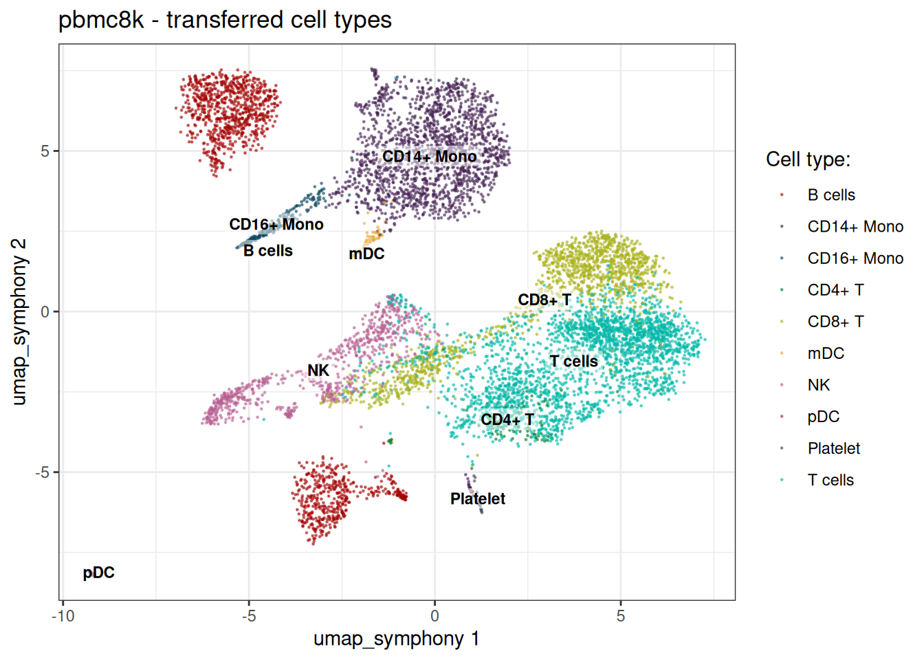
Query UMAP coloured by transferred cell type:
embedding_plot_sc(
  sc_query,
  embedding = "umap_symphony",
  colour_by = "predicted_sc_type",
  label_by = "predicted_sc_type",
  discrete = TRUE
) +
  labs(
    title = "pbmc8k - transferred cell types",
    colour = "Cell type:"
  )
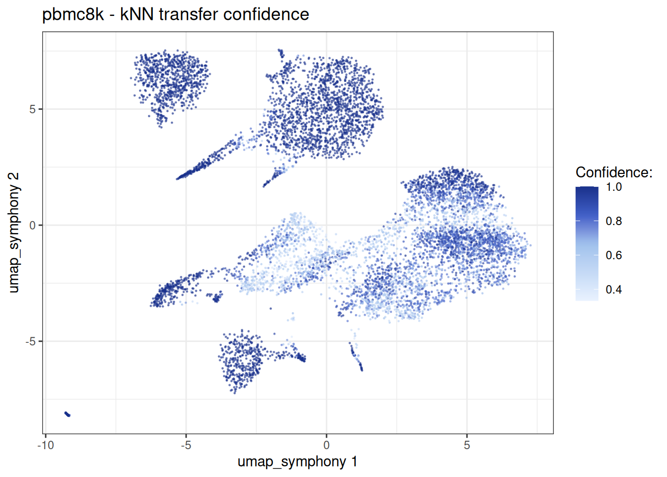
Same UMAP, coloured by transfer confidence. Cells in the interior of their cell type sit at confidence 1; cells on cluster boundaries or in cell types poorly represented in the reference are the ones to scrutinise.
embedding_plot_sc(
  sc_query,
  embedding = "umap_symphony",
  colour_by = "sc_type_confidence",
  discrete = FALSE
) +
  labs(
    title = "pbmc8k - kNN transfer confidence",
    colour = "Confidence:"
  )
And a per-cell-type confidence distribution, useful for spotting cell types where the reference and query disagree systematically:
conf_dt <- sc_query[[c("predicted_sc_type", "sc_type_confidence")]]

ggplot(conf_dt, aes(x = predicted_sc_type, y = sc_type_confidence)) +
  geom_violin(scale = "width", fill = "grey80") +
  geom_jitter(width = 0.15, alpha = 0.2, size = 0.4) +
  labs(
    x = NULL,
    y = "Transfer confidence",
    title = "Per-cell-type kNN agreement on pbmc8k"
  ) +
  theme_minimal() +
  theme(axis.text.x = element_text(angle = 30, hjust = 1)) +
  ylim(0, 1.025)
#> Warning: Removed 112 rows containing missing values or values outside the scale range
#> (`geom_point()`).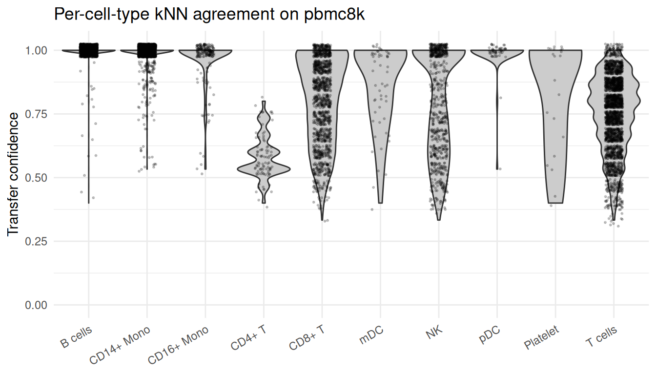
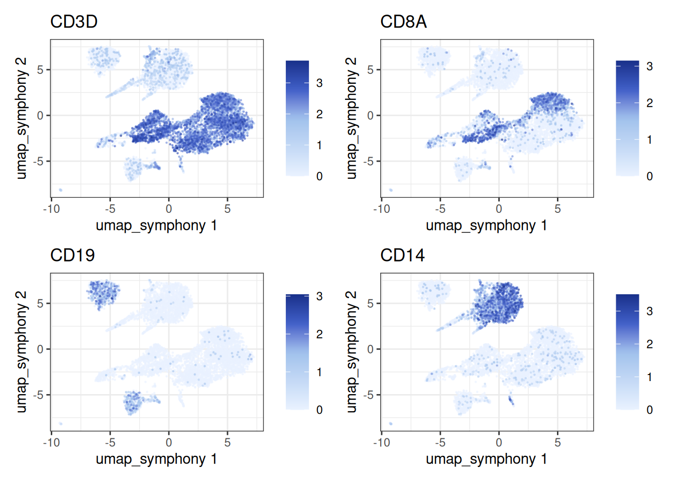
Sanity check of the transferred labels with the canonical markers:
feature_plot_sc(
  object = sc_query,
  features = c(
    "ENSG00000167286",
    "ENSG00000153563",
    "ENSG00000177455",
    "ENSG00000170458"
  ),
  feature_labels = c(
    "ENSG00000167286" = "CD3D",
    "ENSG00000153563" = "CD8A",
    "ENSG00000177455" = "CD19",
    "ENSG00000170458" = "CD14"
  ),
  embedding = "umap_symphony"
)
Slim references and post-hoc labels
The reference above stores z_corr, z_orig, the soft cluster assignments r and the labels. For large references that get checked into shared storage, z_orig and r are dead weight; passing slim = TRUE at build time drops them. z_corr is always retained, since kNN label transfer searches against it.
If you want to add or update labels after the reference is built (say, you re-ran scType with a different marker set), use add_symphony_labels(). It reads obs columns from a SingleCells object in cells_to_keep order and snapshots them into the reference. The cells_to_keep state must match the reference; the function errors if the row count drifts.
slim_ref <- build_symphony_ref(
  object = sc_ref,
  batch_column = "exp_id",
  hvg = hvg_indices,
  harmony_params = params_sc_harmony_v2(),
  pca_params = params_sc_pca(),
  no_pcs = 30L,
  slim = TRUE
)

slim_ref <- add_symphony_labels(
  reference = slim_ref,
  sc_object = sc_ref,
  columns = "sc_type"
)
Multiple label columns can be attached at once (columns = c(...)), existing columns are protected unless you pass overwrite = TRUE, and get_symphony_labels(reference) returns the stored data.table (or NULL if none).