library(bixverse)
library(ggplot2)
library(data.table)
#>
#> Attaching package: 'data.table'
#> The following object is masked from 'package:base':
#>
#>     %notin%
library(bixverse.plots)
library(magrittr)
Sub-clustering and per-group pipelines
2026-09-24
Intro
Your first pass of clustering gives you lineages: T cells, B cells, monocytes. What it does not give you is the structure inside those lineages. The highly variable genes and the principal components were chosen to separate a monocyte from a B cell, and on that axis every T cell looks the same. If you crank up the Leiden resolution on the full object you mostly get the lineages chopped into arbitrary pieces, not naive versus memory CD4.
The fix is to throw the global feature selection away and redo it on the cells you actually care about. That is what SingleCellsSubset is for. It gives you a view onto a subset of a SingleCells object that shares the on-disk counts with the parent, but carries its own empty cache, so HVG, PCA, neighbours and clusters all get recomputed from scratch on the subset alone.
This vignette assumes you have read the design choices and the PBMC walkthrough. The standard chain is not re-explained here.
A coarse first pass
Same PBMC3k data set as the main walkthrough, run through QC, HVG, PCA, neighbours and Leiden without commentary.
pbmc3k_path <- download_pbmc3k()

tempdir_pbmc <- tempdir()

sc_object <- SingleCells(dir_data = tempdir_pbmc)

sc_object <- load_mtx(
  object = sc_object,
  sc_mtx_io_param = get_cell_ranger_params(pbmc3k_path),
  mtx_streaming = FALSE,
  .verbose = FALSE
)

setnames_sc(
  object = sc_object,
  table = "var",
  old = "column1",
  new = "gene_symbol"
)

var <- get_sc_var(sc_object)

ensembl_to_symbol <- setNames(var$gene_symbol, var$gene_id)
symbol_to_ensembl <- setNames(var$gene_id, var$gene_symbol)
Mitochondrial proportions, MAD outliers, cells to keep.
gs_of_interest <- list(
  MT = var[grepl("^MT-", gene_symbol), gene_id]
)

sc_object <- gene_set_proportions_sc(
  sc_object,
  gs_of_interest,
  streaming = FALSE,
  .verbose = FALSE
)

qc_df <- sc_object[[c("cell_id", "lib_size", "nnz", "MT")]]

qc <- run_cell_qc(
  metrics = list(
    log10_lib_size = log10(qc_df$lib_size),
    log10_nnz = log10(qc_df$nnz),
    MT = qc_df$MT
  ),
  cells_to_keep = get_cells_to_keep(sc_object),
  directions = c(
    log10_lib_size = "twosided",
    log10_nnz = "twosided",
    MT = "above"
  ),
  threshold = 3
)

sc_object <- set_cells_to_keep(sc_object, qc_df[!qc$combined, cell_id])
Now the standard chain. The data is tiny, so exhaustive kNN beats building an index.
sc_object <- find_hvg_sc(sc_object, hvg_no = 2000L, .verbose = FALSE)

sc_object <- calculate_pca_sc(
  object = sc_object,
  no_pcs = 30L,
  sparse_svd = TRUE,
  .verbose = FALSE
)

sc_object <- find_neighbours_sc(
  object = sc_object,
  neighbours_params = params_sc_neighbours(
    knn = list(knn_method = "exhaustive")
  ),
  .verbose = FALSE
)

sc_object <- find_clusters_sc(sc_object, res = 1, name = "leiden_global")

sc_object <- umap_sc(sc_object, .verbose = FALSE)
For the annotation we deliberately stay coarse. No CD4 versus CD8 split, no naive versus memory. Lineage only, because the fine structure is exactly what we want the subset to recover.
coarse_markers <- c(
  CD3D = "T cells",
  CD3E = "T cells",
  CD3G = "T cells",
  TRAC = "T cells",
  MS4A1 = "B cells",
  CD79A = "B cells",
  CD19 = "B cells",
  CD14 = "Monocytes",
  LYZ = "Monocytes",
  S100A8 = "Monocytes",
  FCGR3A = "Monocytes",
  GNLY = "NK",
  NKG7 = "NK",
  KLRD1 = "NK",
  FCER1A = "DC",
  CD1C = "DC",
  LILRA4 = "DC",
  PPBP = "Platelet",
  PF4 = "Platelet"
)

coarse_dt <- stack(coarse_markers) %>%
  as.data.table() %>%
  setnames(., c("values", "ind"), c("cell_type", "gene_symbol")) %>%
  .[, gene_symbol := as.character(gene_symbol)] %>%
  .[, gene_id := var$gene_id[match(gene_symbol, var$gene_symbol)]] %>%
  .[!is.na(gene_id), ]

sctype_scores <- calc_sc_type_scores(
  object = sc_object,
  cell_marker_list = prepare_cell_markers(sc_object, coarse_dt)
)

cell_type_anno <- score_clusters(
  sctype_scores,
  sc_object[[]][["leiden_global"]]
)

obs <- get_sc_obs(sc_object, filtered = TRUE)

sc_object[["cell_type"]] <- cell_type_anno$cell_type[match(
  obs$leiden_global,
  cell_type_anno$cluster_id
)]

get_sc_obs(sc_object, filtered = TRUE)[, .N, by = cell_type][order(-N)]
#>    cell_type     N
#>       <char> <int>
#> 1:   T cells  1046
#> 2: Monocytes   458
#> 3:        NK   379
#> 4:   B cells   280
embedding_plot_sc(
  sc_object,
  embedding = "umap",
  colour_by = "cell_type",
  label_by = "cell_type",
  discrete = TRUE
) +
  labs(colour = "Cell type")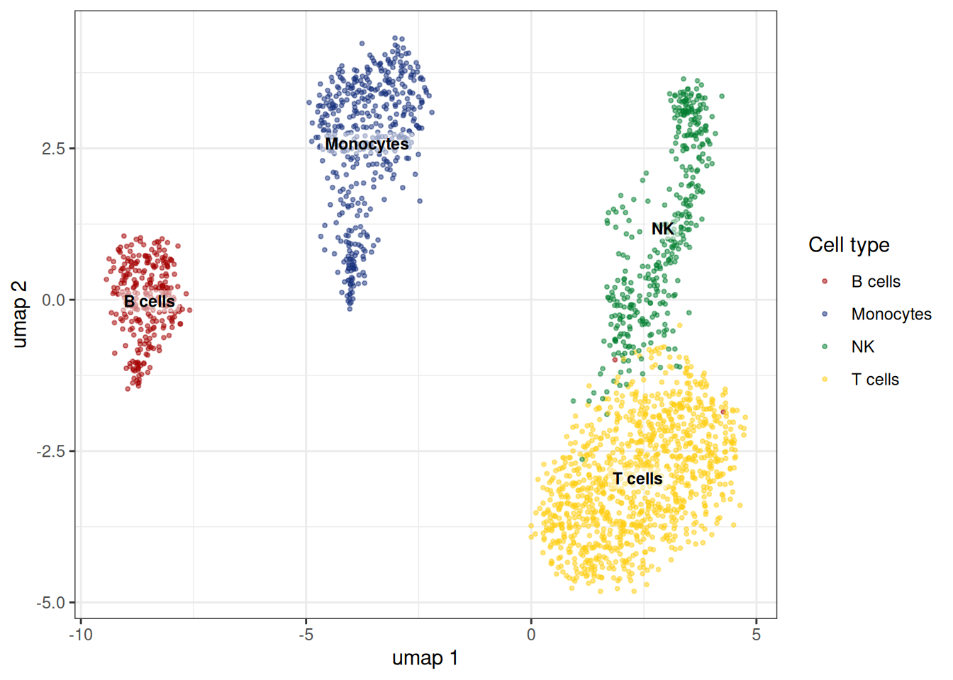
Taking a subset
The constructor takes the parent, a column in obs, and the level you want.
t_cells <- SingleCellsSubset(
  sc_object = sc_object,
  grouping_column = "cell_type",
  group = "T cells"
)

t_cells
#> Single cell experiment (subset).
#>   No cells: 1046
#>   No genes: 11139
#>   Group: cell_type = T cells
#>   HVG calculated: FALSE
#>   PCA calculated: FALSE
#>   Other embeddings: none
#>   KNN generated: FALSE
#>   SNN generated: FALSE
#>   Stale artefacts: none
The print method tells you the important bit: HVG, PCA, kNN and sNN are all FALSE. Nothing was inherited. The subset shares the Rust count connection with the parent, so no counts were copied and no files were written, but the ScCache is brand new and the parent’s HVG selection was dropped on purpose.
Everything else behaves like the parent object. The obs table is filtered to the group, the var table is untouched, and the usual getters work.
dim(t_cells)
#> [1]  1046 11139

head(t_cells)[, .(cell_id, cell_idx, lib_size, cell_type)]
#>             cell_id cell_idx lib_size cell_type
#>              <char>    <num>    <num>    <char>
#> 1: AAACATACAACCAC-1        1     2418   T cells
#> 2: AAACATTGATCAGC-1        3     3144   T cells
#> 3: AAACGCACTGGTAC-1        6     2154   T cells
#> 4: AAACTTGATCCAGA-1       12     2382   T cells
#> 5: AAAGAGACGAGATA-1       13     2403   T cells
#> 6: AAAGCCTGTATGCG-1       20     2922   T cells
A note on indices
This is the one place where you can shoot yourself in the foot, so it is worth being explicit. The subset keeps two index spaces around:
-
Subset positions are 1-indexed rows of the subset’s own obs table. This is what
[and[[take. -
Original positions are the parent’s index space.
subset_to_originaland thecell_idxobs column both hold these, 1-indexed. Everything that reaches Rust gets translated into this space, 0-indexed, before the call.
get_cell_indices() lets you ask for either.
first_three <- get_cell_names(t_cells)[1:3]

# 1-indexed position within the subset
get_cell_indices(t_cells, cell_ids = first_three, rust_index = FALSE)
#> [1] 1 2 3

# 0-indexed position in the parent, which is what Rust sees
get_cell_indices(t_cells, cell_ids = first_three, rust_index = TRUE)
#> [1] 0 2 5
The practical upshot: you never translate manually. Hand cell IDs or subset positions to the getters and let the class deal with it. The cell_idx column is there so you can join results back onto the parent later, which is exactly what we do further down.
Re-running the chain
Same functions as on the parent. They dispatch on the subset.
t_cells <- find_hvg_sc(t_cells, hvg_no = 2000L, .verbose = FALSE)

t_cells <- calculate_pca_sc(
  object = t_cells,
  no_pcs = 20L,
  sparse_svd = TRUE,
  .verbose = FALSE
)

t_cells <- find_neighbours_sc(
  object = t_cells,
  neighbours_params = params_sc_neighbours(
    knn = list(knn_method = "exhaustive")
  ),
  .verbose = FALSE
)

t_cells <- find_clusters_sc(t_cells, res = 0.5, name = "t_subcluster")

t_cells <- umap_sc(t_cells, .verbose = FALSE)

t_cells
#> Single cell experiment (subset).
#>   No cells: 1046
#>   No genes: 11139
#>   Group: cell_type = T cells
#>   HVG calculated: TRUE
#>   PCA calculated: TRUE
#>   Other embeddings: umap
#>   KNN generated: TRUE
#>   SNN generated: TRUE
#>   Stale artefacts: none
Was any of that worth it? Check how much the feature selection actually moved.
Around a thousand of the 2000 genes are different, and the ones that dropped out are the monocyte and B cell markers that were carrying the global PCA. The subset PCA is built on genes that vary within T cells, which is the whole point.
embedding_plot_sc(
  t_cells,
  embedding = "umap",
  colour_by = "t_subcluster",
  label_by = "t_subcluster",
  discrete = TRUE
) +
  labs(colour = "Sub-cluster")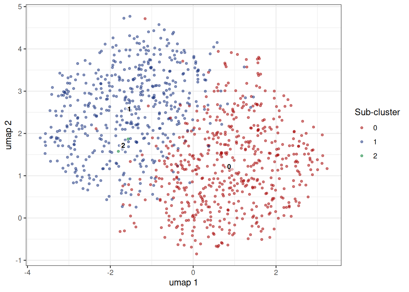
Markers for the sub-clusters
Differential expression dispatches on the subset, so the comparison is automatically confined to it. Each sub-cluster is tested against the other T sub-clusters, not against every monocyte in the data set.
sub_markers <- find_all_markers_sc(
  object = t_cells,
  column_of_interest = "t_subcluster",
  .verbose = FALSE
)

sub_markers[, gene_symbol := ensembl_to_symbol[gene_id]]

sub_markers[fdr <= 0.05][order(grp, -lfc)][,
  head(.SD, 5),
  by = grp,
  .SDcols = c("gene_symbol", "lfc", "fdr")
]
#>       grp        gene_symbol       lfc          fdr
#>     <int>             <char>     <num>        <num>
#>  1:     0             S100A4 1.5171083 5.137542e-85
#>  2:     0              ANXA1 0.8223093 5.096615e-29
#>  3:     0            S100A11 0.8210568 3.329714e-34
#>  4:     0               KLF6 0.7815999 9.624673e-26
#>  5:     0           SH3BGRL3 0.7646732 7.046937e-33
#>  6:     1               CCR7 0.5379487 9.096949e-19
#>  7:     1            C6orf48 0.3903745 3.988756e-10
#>  8:     1               CD8B 0.3675649 3.410456e-10
#>  9:     1              RPS3A 0.3314095 1.408217e-26
#> 10:     1               BTG1 0.3313620 2.968827e-11
#> 11:     2 XXbac-BPG299F13.17 2.9109616 8.112309e-03
#> 12:     2             FCER1A 2.8321912 2.592287e-41
#> 13:     2              LZTS2 2.5425797 1.346397e-11
#> 14:     2               GPX1 2.4119055 1.028758e-02
#> 15:     2              USP30 2.3417146 1.092048e-22
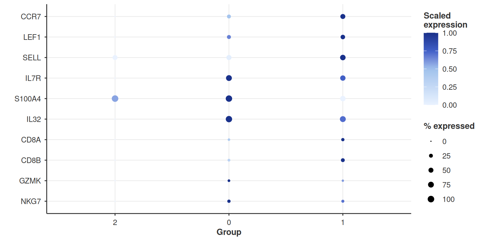
S100A4, ANXA1 and IL32 on one side, CCR7, SELL and CD8B on the other. That is the memory versus naive split, and the global clustering had no way of seeing it. Cluster 2 is two cells, which is Leiden being Leiden at this resolution.
The expression plots work on the subset too, so you can go straight to a dot plot without touching the parent.
t_features <- setdiff(
  symbol_to_ensembl[c(
    "CCR7",
    "LEF1",
    "SELL",
    "IL7R",
    "S100A4",
    "IL32",
    "CD8A",
    "CD8B",
    "GZMK",
    "NKG7"
  )],
  NA
)

dot_plot_sc(
  object = t_cells,
  features = t_features,
  feature_labels = ensembl_to_symbol[t_features],
  grouping_variable = "t_subcluster",
  scale_exp = TRUE,
  cluster_groups = TRUE
)
Getting the labels back to the parent
So far everything lives in the subset, in memory. To make the labels permanent, or to plot them on the parent’s global UMAP, push them into the parent’s DuckDB. merge_subset_obs() does the join on cell_idx for you.
sc_object <- merge_subset_obs(
  object = sc_object,
  subsets = t_cells,
  cols = "t_subcluster",
  prefix_values = TRUE
)
#> Merged 1 column(s) for 1046 cells into obs (1654 cells left as NA).

get_sc_obs(sc_object, filtered = TRUE)[, .N, by = t_subcluster][order(
  t_subcluster
)]
#>    t_subcluster     N
#>          <char> <int>
#> 1:    T cells_0   554
#> 2:    T cells_1   490
#> 3:    T cells_2     2
#> 4:         <NA>  1117
prefix_values = TRUE stamps the subset’s group onto every value, so you get T cells_0 rather than a bare 0. Drop it if you want the raw labels. Leave cols out and everything the subset gained that the parent does not have yet gets merged, which after a pipeline run is exactly the new columns.
The join is a left join, so every cell that was not a T cell gets NA. That is the behaviour you want, and the downstream methods respect it.
Results that already carry their own cell_idx skip the helper entirely. fast_cluster_sc() returns memberships keyed in parent space, so add_sc_new_obs() takes them directly.
fast_sub <- fast_cluster_sc(
  object = t_cells,
  resolutions = c(1, 0.5),
  .verbose = FALSE
)

sc_object <- add_sc_new_obs(sc_object, get_data(fast_sub))

head(sc_object)[, .(cell_id, cell_type, t_subcluster, res_1, res_0.5)]
#>             cell_id cell_type t_subcluster res_1 res_0.5
#>              <char>    <char>       <char> <int>   <int>
#> 1: AAACATACAACCAC-1   T cells    T cells_0     0       0
#> 2: AAACATTGATCAGC-1   T cells    T cells_0     0       0
#> 3: AAACCGTGCTTCCG-1 Monocytes         <NA>    NA      NA
#> 4: AAACGCACTGGTAC-1   T cells    T cells_0     0       0
#> 5: AAACGCTGGTTCTT-1        NK         <NA>    NA      NA
#> 6: AAACGCTGTAGCCA-1        NK         <NA>    NA      NA
Pipelines
Once you are doing this for more than one cell type, writing out HVG, PCA, neighbours and clusters by hand five times gets old. sc_pipeline() lets you declare the chain once.
subcluster_pipeline <- sc_pipeline() %>>%
  step_hvg_sc(hvg_no = 2000L, .verbose = FALSE) %>>%
  step_pca_sc(no_pcs = 20L, sparse_svd = TRUE, .verbose = FALSE) %>>%
  step_neighbours_sc(
    neighbours_params = params_sc_neighbours(
      knn = list(knn_method = "exhaustive")
    ),
    .verbose = FALSE
  ) %>>%
  step_clusters_sc(res = 0.5, name = "subcluster")

subcluster_pipeline
#> <ScPipeline> 4 steps
#>   1. hvg         hvg_no = 2000L, hvg_params = <list>, streaming = NULL, .verbose = FALSE
#>   2. pca         no_pcs = 20L, pca_params = <list>, sparse_svd = TRUE, hvg = NULL, seed = 42L, .verbose = FALSE
#>   3. neighbours  embd_to_use = "pca", no_embd_to_use = NULL, modality = c("rna", "adt"), neighbours_params = <list>, seed = 42L, .verbose = FALSE
#>   4. clusters    cluster_algorithm = c("leiden", "louvain"), res = 0.5, name = "subcluster", modality = c("rna", "adt", "wnn"), seed = 42L
Pipelines are inert. Nothing runs until you apply one, and the same pipeline works on a SingleCells or a SingleCellsSubset because dispatch happens inside each step.
b_cells <- SingleCellsSubset(
  sc_object = sc_object,
  grouping_column = "cell_type",
  group = "B cells"
)

b_cells <- apply_pipeline(subcluster_pipeline, b_cells)

b_cells
#> Single cell experiment (subset).
#>   No cells: 280
#>   No genes: 11139
#>   Group: cell_type = B cells
#>   HVG calculated: TRUE
#>   PCA calculated: TRUE
#>   Other embeddings: none
#>   KNN generated: TRUE
#>   SNN generated: TRUE
#>   Stale artefacts: none
One pipeline, every group
apply_pipeline_per_group() builds the subset for you and returns a named list.
Sizing matters here. PCA with 20 components needs more than 20 cells, so a rare population that the annotation happened to call will fall over and take the whole run with it. Restrict the groups explicitly rather than hoping for the best. On this data set the coarse annotation only returned four lineages and all of them clear the bar, so nothing gets dropped, but the guard costs nothing.
cell_counts <- get_sc_obs(sc_object, filtered = TRUE)[, .N, by = cell_type][
  order(-N)
]

groups_to_run <- cell_counts[N >= 100, cell_type]

groups_to_run
#> [1] "T cells"   "Monocytes" "NK"        "B cells"
per_group <- apply_pipeline_per_group(
  pipeline = subcluster_pipeline,
  object = sc_object,
  group_col = "cell_type",
  groups = groups_to_run
)

summary_dt <- data.table::rbindlist(purrr::imap(per_group, \(x, name) {
  data.table(
    cell_type = name,
    n_cells = dim(x)[1],
    n_subclusters = length(unique(get_sc_obs(x)$subcluster)),
    hvg_shared_with_global = length(intersect(get_hvg(x), global_hvg))
  )
}))

summary_dt[order(-n_cells)]
#>    cell_type n_cells n_subclusters hvg_shared_with_global
#>       <char>   <int>         <int>                  <int>
#> 1:   T cells    1046             3                   1016
#> 2: Monocytes     458             2                    820
#> 3:        NK     379             3                    669
#> 4:   B cells     280             1                    581
Every lineage picked a different feature set, and the shared fraction with the global HVGs is nowhere near complete. Running one global PCA and hoping it resolves everything was never going to work.
Writing all of that back is one call. merge_subset_obs() takes the list straight from apply_pipeline_per_group(), checks that no cell shows up twice, and does a single join.
sc_object <- merge_subset_obs(
  object = sc_object,
  subsets = per_group,
  cols = "subcluster",
  new_names = "fine_label",
  prefix_values = TRUE
)
#> Merged 1 column(s) for 2163 cells into obs (537 cells left as NA).

get_sc_obs(sc_object, filtered = TRUE)[, .N, by = fine_label][order(fine_label)]
#>     fine_label     N
#>         <char> <int>
#> 1:   B cells_0   280
#> 2: Monocytes_0   233
#> 3: Monocytes_1   225
#> 4:        NK_0   138
#> 5:        NK_1   128
#> 6:        NK_2   113
#> 7:   T cells_0   554
#> 8:   T cells_1   490
#> 9:   T cells_2     2
The prefix is doing real work here. Every group’s Leiden run starts counting at zero, so without it the T cell 1 and the B cell 1 collapse into one label. Leave it out and you get a warning naming the values that clash.
embedding_plot_sc(
  sc_object,
  embedding = "umap",
  colour_by = "fine_label",
  discrete = TRUE
) +
  labs(colour = "Fine label")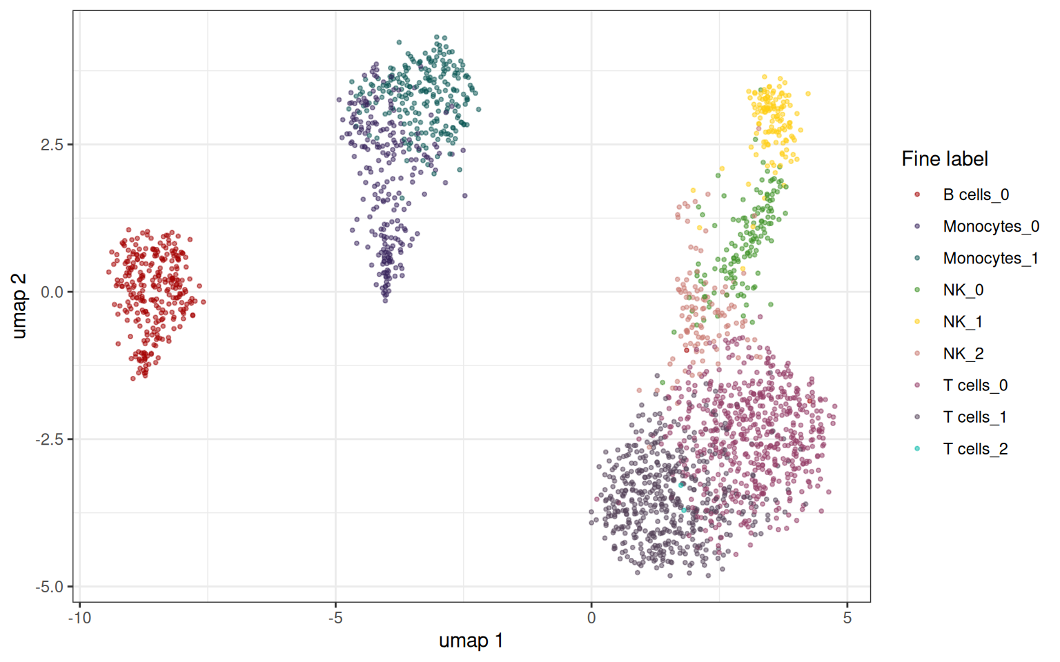
Source-pure meta cells
All three meta cell generators run on a subset, so you can aggregate per patient and never mix two donors into one meta cell. The catch used to be the last step: you ended up with one MetaCells object per patient and no way to run SCENIC or NMF across the lot. merge_meta_cells() closes that.
step_metacells_sc() puts the generation into the chain itself. It is the one step that changes the class of the object, so a pipeline that ends on it hands you MetaCells rather than SingleCellsSubset. Everything before it still runs per patient, which is the point when your samples are split over two plates and need correcting within a donor.
mc_pipeline <- sc_pipeline() %>>%
  step_hvg_sc(hvg_no = 2000L) %>>%
  step_pca_sc(no_pcs = 20L) %>>%
  step_harmony_sc(batch_column = "plate") %>>%
  step_neighbours_sc(embd_to_use = "harmony") %>>%
  step_metacells_sc(
    "bootstrapped",
    sc_meta_cell_params = params_sc_bt_metacells(target_no_metacells = 100L)
  )

per_patient <- apply_pipeline_per_group(
  pipeline = mc_pipeline,
  object = sc_object,
  group_col = "patient_id"
)

meta_cells <- merge_meta_cells(per_patient)
A few things worth knowing:
-
meta_cells_per_group()does the whole thing in one call if you do not need the per-patient objects. Same arguments, plusmethodandmc_params. - The merged obs table gains a
source_idcolumn and the meta cell ids are prefixed with it.original_cell_idxstays in the index space of its own source, so it is only meaningful alongsidesource_id. - Gene spaces are reconciled by
intersect(the default) orunion, the latter zero-filling genes an input lacks. Both are no-ops when every input came from the same parent object. - Counts are carried over untouched. Normalisation is per meta cell, so row-binding leaves it valid.
- PCA, kNN, sNN and HVG are dropped on merge. They were fitted per patient and mean nothing side by side. Recompute them on the merged object, which is the whole reason for merging.
-
validate_pipeline()checks a chain against a starting class before anything runs.apply_pipeline()andapply_pipeline_per_group()call it for you, so puttingstep_harmony_sc()afterstep_metacells_sc()errors immediately instead of after twenty minutes of PCA.
Caveats and what is next
A few sharp edges to be aware of before you build on this.
Meta cell memberships come back as positions in the parent obs table, which is what makes them joinable back onto the original object. get_pseudobulked_sc() runs on subsets too if aggregation is all you are after.
Subsets are RNA only. If you hand modality = "adt" to a getter you get an error, so multi-modal work stays on SingleCellsMultiModal.
Subsets nest conceptually but not in code: you cannot build a SingleCellsSubset from another SingleCellsSubset. If you want a third level, write the labels back to the parent and subset from there.
Clean up
unlink(tempdir_pbmc, recursive = TRUE, force = TRUE)