library(bixverse)
library(bixverse.plots)
library(data.table)
#>
#> Attaching package: 'data.table'
#> The following object is masked from 'package:base':
#>
#>     %notin%
library(ggplot2)
Ambient RNA removal with CellSweep
2026-09-24
Intro
Cells lyse during dissociation and their transcripts end up in the buffer. Every droplet then gets loaded with a bit of that soup on top of whatever cell it caught, which is why you find monocyte genes in T cells, haemoglobin everywhere, and lineage markers that refuse to be clean. That background is the ambient RNA.
CellSweep attacks it as a mixture problem. Every observed count in a barcode comes from one of three places: the ambient profile of that emulsion, a global bulk profile, or the barcode’s own cell type profile. An EM fit splits the counts three ways per barcode, and subtracting the first two components leaves the denoised matrix. The per-barcode ambient fraction, alpha, falls out of the same fit, which doubles as a quality metric: a barcode that is 60% soup is not a cell you want in your clustering.
Two things about where this sits in a workflow, because both are easy to get wrong.
It runs after annotation, not before. The model subtracts against cell type profiles, so it needs the labels on input. The chain is: ingest the raw barcodes, cluster and annotate as usual, then cellsweep_sc(), then redo the feature selection and reduction on the clean counts.
It needs the empty droplets. The ambient profile is estimated from their pooled counts, and they stay in the EM with their contamination fraction pinned at 1. So the object has to be ingested permissively. The load-time cutoffs in bixverse are irreversible, and the defaults delete exactly the barcodes the model trains on.
The raw matrix
We use the 10x Genomics 5’ PBMC 1k run, the same data the CellSweep reference notebook works through. This is the unfiltered matrix, so every barcode the sequencer saw is in there.
h5_path <- download_pbmc_1k_5p(quiet = FALSE)

meta <- read_tenx_h5_metadata(h5_path)
meta$dims
#>    obs    var
#> 737280  36620
meta$feature_types
#> Antibody Capture  Gene Expression
#>               19            36601
737,280 barcodes and 36,620 features, of which 19 are Antibody Capture. Only the gene expression ones are wanted here, which is what feature_type selects.
Now the permissive load. min_lib_size = 1L throws away the barcodes that saw no molecule at all, which is most of them, and keeps everything else.
tempdir_cellsweep <- file.path(tempdir(), "cellsweep_bixverse")
dir_raw <- file.path(tempdir_cellsweep, "raw")
dir.create(dir_raw, showWarnings = FALSE, recursive = TRUE)

raw_object <- load_tenx_h5(
  object = SingleCells(dir_data = dir_raw),
  h5_path = h5_path,
  sc_qc_param = params_sc_min_quality(
    min_unique_genes = 0L,
    min_lib_size = 1L,
    min_cells = 0L
  ),
  feature_type = "Gene Expression",
  .verbose = TRUE
)
#>  Using light streaming for the CSR to CSC conversion.
#> Loading barcodes from 10x h5 into the DuckDB.
#> Loading features from 10x h5 into the DuckDB.

raw_object
#> Single cell experiment (Single Cells).
#>   No cells (original): 97998
#>    To keep n: 97998
#>   No genes: 36601
#>   HVG calculated: FALSE
#>   PCA calculated: FALSE
#>   Other embeddings: none
#>   KNN generated: FALSE
#>   SNN generated: FALSE
#>   MAGIC imputed: none
#>   Residual model: none
#>   Stale artefacts: none
98k barcodes carrying at least one UMI. The vast majority are empty droplets and that is the point: they are the training data for the soup.
Calling the empty droplets
params_sc_empty_droplets() offers four ways to decide which barcode is empty, in descending order of how much you should trust them. "supplied" takes an existing logical column from the obs table, and if you have Cell Ranger’s filtered barcode list you already know the answer. The other three infer it from the library sizes alone.
The barcode rank curve is the thing they are all trying to read.
obs_raw <- get_sc_obs(raw_object, filtered = FALSE)

rank_dt <- data.table(lib_size = obs_raw$lib_size)
setorder(rank_dt, -lib_size)
rank_dt[, rank := .I]

ggplot(rank_dt, aes(x = rank, y = lib_size)) +
  geom_line(linewidth = 0.7) +
  geom_hline(yintercept = 257, colour = "firebrick", linetype = "dashed") +
  scale_x_log10() +
  scale_y_log10() +
  labs(
    x = "Barcode rank",
    y = "Library size",
    title = "Barcode rank curve",
    subtitle = "Dashed line: the 257 UMI cutoff the reference notebook uses"
  ) +
  theme_minimal()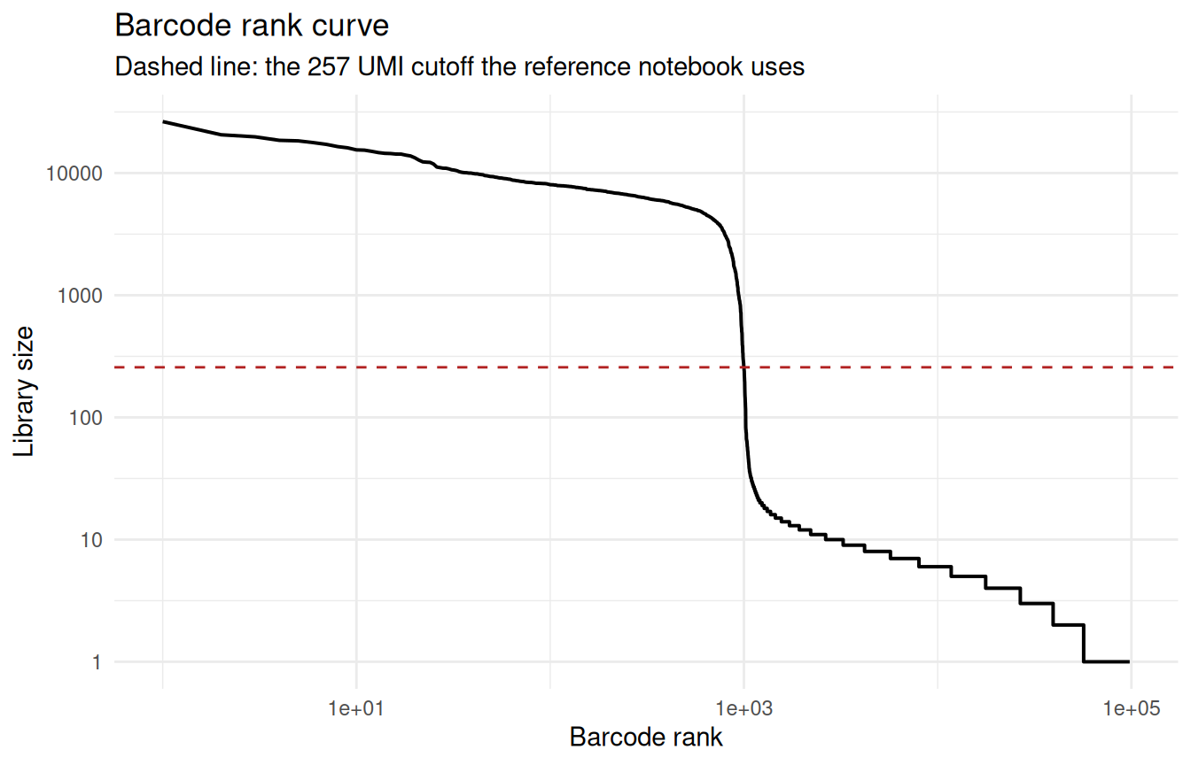
The cliff is obvious. Roughly a thousand barcodes sit well above it and everything else falls off to single-digit libraries.
rs_sc_infer_empty_droplets() is the Rust side of the three inference methods, exposed so the calls can be compared before committing to one.
methods <- list(
  umi_cutoff = params_sc_empty_droplets(
    method = "umi_cutoff",
    umi_cutoff = 257L
  ),
  expected_cells = params_sc_empty_droplets(
    method = "expected_cells",
    expected_cells = 1000L
  ),
  knee = params_sc_empty_droplets(method = "knee")
)

comparison <- rbindlist(purrr::imap(methods, \(params, name) {
  call <- rs_sc_infer_empty_droplets(
    lib_size = as.integer(obs_raw$lib_size),
    empty_params = unclass(params)
  )
  data.table(
    method = name,
    empty = sum(call),
    kept = sum(!call),
    min_kept_lib_size = min(obs_raw$lib_size[!call])
  )
}))

comparison
#>            method empty  kept min_kept_lib_size
#>            <char> <int> <int>             <num>
#> 1:     umi_cutoff 96998  1000               257
#> 2: expected_cells 96998  1000               257
#> 3:           knee 96979  1019               120
umi_cutoff and expected_cells land on the same thousand barcodes, which they should: the cutoff the notebook quotes is the one you get by asking for a thousand cells. The knee detector stops at 120 UMIs instead of 257 and hands back 19 extra barcodes. It is experimental in the reference too, so treat it as a starting point rather than an answer.
We go with the cutoff.
empty_params <- params_sc_empty_droplets(
  method = "umi_cutoff",
  umi_cutoff = 257L
)
Annotating the real cells
CellSweep needs cell type labels, so the real barcodes have to go through a normal pipeline first. The raw object is not the place to do that, since 97k of its barcodes are soup. Load the same file a second time with QC that means something, and cluster there.
dir_cells <- file.path(tempdir_cellsweep, "cells")

dir.create(dir_cells, showWarnings = FALSE, recursive = TRUE)

cell_object <- load_tenx_h5(
  object = SingleCells(dir_data = dir_cells),
  h5_path = h5_path,
  sc_qc_param = params_sc_min_quality(
    min_unique_genes = 200L,
    min_lib_size = 257L,
    min_cells = 3L
  ),
  feature_type = "Gene Expression",
  .verbose = TRUE
)
#>  Using light streaming for the CSR to CSC conversion.
#> Loading barcodes from 10x h5 into the DuckDB.
#> Loading features from 10x h5 into the DuckDB.

cell_object
#> Single cell experiment (Single Cells).
#>   No cells (original): 975
#>    To keep n: 975
#>   No genes: 15015
#>   HVG calculated: FALSE
#>   PCA calculated: FALSE
#>   Other embeddings: none
#>   KNN generated: FALSE
#>   SNN generated: FALSE
#>   MAGIC imputed: none
#>   Residual model: none
#>   Stale artefacts: none
Standard QC on top: mitochondrial fraction, then MAD-based outlier detection across the usual three metrics.
var_cells <- get_sc_var(cell_object)

cell_object <- gene_set_proportions_sc(
  cell_object,
  gene_set_list = list(MT = var_cells[grepl("^MT-", gene_name), gene_id]),
  streaming = FALSE,
  .verbose = FALSE
)

qc_df <- cell_object[[c("cell_id", "lib_size", "nnz", "MT")]]

qc <- run_cell_qc(
  metrics = list(
    log10_lib_size = log10(qc_df$lib_size),
    log10_nnz = log10(qc_df$nnz),
    MT = qc_df$MT
  ),
  cells_to_keep = get_cells_to_keep(cell_object),
  directions = c(
    log10_lib_size = "twosided",
    log10_nnz = "twosided",
    MT = "above"
  ),
  threshold = 3
)

cell_object <- set_cells_to_keep(cell_object, qc_df[!qc$combined, cell_id])

sum(qc$combined)
#> [1] 213
Then the pipeline, unchanged from any other single cell workflow.
cell_object <- find_hvg_sc(cell_object, hvg_no = 2000L, .verbose = FALSE)

cell_object <- calculate_pca_sc(
  cell_object,
  no_pcs = 30L,
  sparse_svd = TRUE,
  .verbose = FALSE
)

cell_object <- find_neighbours_sc(
  cell_object,
  neighbours_params = params_sc_neighbours(
    knn = list(knn_method = "exhaustive")
  ),
  .verbose = FALSE
)

cell_object <- find_clusters_sc(
  cell_object,
  res = 1,
  name = "leiden_clusters"
)

obs_cells <- get_sc_obs(cell_object)

table(obs_cells$leiden_clusters)
#>
#>   0   1   2   3   4   5   6   7
#> 217 189  98  85  69  39  35  30
762 cells over eight clusters. Good enough to subtract against; you would name them with calc_sc_type_scores() or a reference in a real analysis, but the model only cares that barcodes with the same label share a profile.
Putting the labels back
The labels live on the cell object and CellSweep reads them off the raw one, so they have to be joined across by barcode. Every barcode that is not a clustered cell keeps an NA, which is exactly how cellsweep_sc() finds the barcodes it should ignore.
label <- obs_cells$leiden_clusters[
  match(obs_raw$cell_id, obs_cells$cell_id)
]

cell_type <- rep(NA_character_, nrow(obs_raw))
cell_type[!is.na(label)] <- sprintf("cluster_%s", label[!is.na(label)])

raw_object[["cell_type"]] <- cell_type
raw_object[["sample_id"]] <- rep("pbmc_1k", nrow(obs_raw))

table(cell_type, useNA = "ifany")
#> cell_type
#> cluster_0 cluster_1 cluster_2 cluster_3 cluster_4 cluster_5 cluster_6 cluster_7
#>       217       189        98        85        69        39        35        30
#>      <NA>
#>     97236
Watch the NA handling there. sprintf("cluster_%s", NA) gives you the string "cluster_NA", and CellSweep will happily treat those barcodes as a ninth cell type and fit a profile to them. Keep the NA an NA.
sample_id is a constant here because this is one emulsion. It is still required: the ambient profile is a property of a single run, and pooling samples into one profile is wrong even when it runs.
Running CellSweep
dir_clean <- file.path(tempdir_cellsweep, "clean")
dir.create(dir_clean, showWarnings = FALSE, recursive = TRUE)

clean_object <- cellsweep_sc(
  target = SingleCells(dir_data = dir_clean),
  input = raw_object,
  celltype_column = "cell_type",
  sample_column = "sample_id",
  empty_params = empty_params,
  .verbose = TRUE
)
#> Empty droplets (method 'umi_cutoff'): 96_998 of 97_998 barcodes called empty.
#> 238 barcodes are neither empty nor annotated-and-passing-QC. They are excluded from the fit and from the output.
#> Running CellSweep over 1 samples, 762 barcodes, 96998 empty droplets.
#> Generating gene-based binary.
#> Populating obs and var tables.

clean_object
#> Single cell experiment (Single Cells).
#>   No cells (original): 762
#>    To keep n: 762
#>   No genes: 36601
#>   HVG calculated: FALSE
#>   PCA calculated: FALSE
#>   Other embeddings: none
#>   KNN generated: FALSE
#>   SNN generated: FALSE
#>   MAGIC imputed: none
#>   Residual model: none
#>   Stale artefacts: none
Three numbers in that output are worth reading. 96,998 barcodes went into the ambient profile. 762 got denoised. And 238 barcodes were neither: they cleared the UMI cutoff but failed QC or the outlier check, so they have no label to subtract against. Those are dropped from the fit and from the output, which is why the clean object is 762 cells and not 1000.
The denoised counts land in a new directory. The raw layer takes stochastically rounded values so the negative binomial methods downstream still see integers, and the normalised layer keeps the float magnitudes.
What came out
The ambient profile is the first thing to look at, because it is the one part of the fit you can sanity check against what you know about the tissue.
var_clean <- get_sc_var(clean_object)

top_ambient <- var_clean[order(-cellsweep_ambient)][1:20]

ggplot(
  top_ambient,
  aes(x = cellsweep_ambient, y = reorder(gene_name, cellsweep_ambient))
) +
  geom_col(fill = "steelblue") +
  labs(
    x = "Fraction of the ambient profile",
    y = NULL,
    title = "What the soup is made of"
  ) +
  theme_minimal()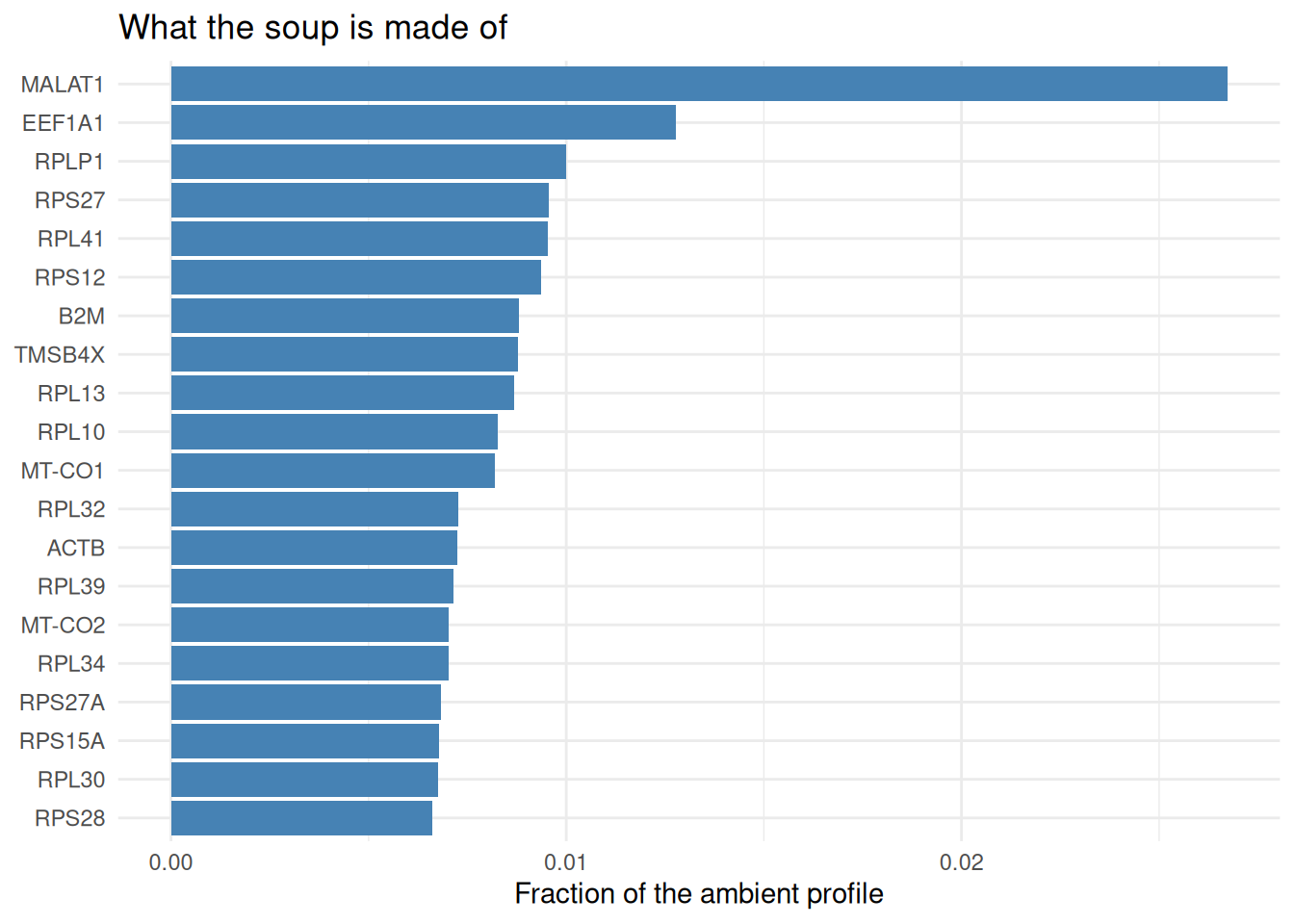
MALAT1, elongation factors, ribosomal proteins, B2M, mitochondrial genes. That is the soup of a lysing PBMC and nothing else, which is a good sign.
Next, the per-barcode contamination.
obs_clean <- get_sc_obs(clean_object, filtered = FALSE)

ggplot(obs_clean, aes(x = cellsweep_alpha)) +
  stat_ecdf(linewidth = 0.7) +
  geom_vline(xintercept = 0.3, colour = "firebrick", linetype = "dashed") +
  labs(
    x = "Estimated ambient fraction",
    y = "Cumulative fraction of cells",
    title = "How much soup each barcode carries"
  ) +
  theme_minimal()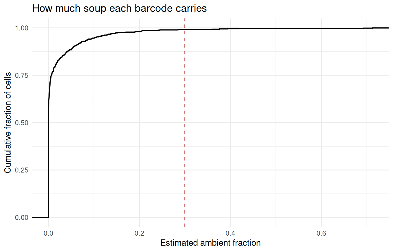
summary(obs_clean$cellsweep_alpha)
#>      Min.   1st Qu.    Median      Mean   3rd Qu.      Max.
#> 0.000e+00 1.010e-06 1.094e-04 1.880e-02 6.568e-03 7.126e-01

obs_clean[,
  .(n = .N, median_alpha = median(cellsweep_alpha)),
  by = cell_type
][order(-median_alpha)]
#>    cell_type     n median_alpha
#>       <char> <int>        <num>
#> 1: cluster_1   189 1.052427e-02
#> 2: cluster_2    98 1.847317e-04
#> 3: cluster_0   217 8.382157e-05
#> 4: cluster_3    85 1.983908e-05
#> 5: cluster_5    39 1.802193e-05
#> 6: cluster_7    30 1.845909e-06
#> 7: cluster_6    35 4.589875e-07
#> 8: cluster_4    69 3.052440e-07
This run is clean. The median barcode is essentially uncontaminated and only a handful sit above the 0.3 the reference notebook filters at. That is not always what you get, and it is worth knowing before you assume your lineage markers are real.
Does the subtraction do anything?
The honest test is not whether alpha looks plausible but whether the counts change in the direction they should. Monocyte genes appearing in T cells are soup by construction, so track a couple of them across clusters, before and after.
markers <- c("LYZ" = "monocyte", "S100A8" = "monocyte", "PPBP" = "platelet")
marker_ids <- var_clean[gene_name %in% names(markers), gene_id]
names(marker_ids) <- var_clean[gene_name %in% names(markers), gene_name]

detection_rate <- function(object, layer_name) {
  expr <- extract_gene_expression(
    object,
    features = marker_ids,
    obs_cols = c("cell_id", "cell_type")
  )
  setDT(expr)
  expr <- expr[!is.na(cell_type)]
  long <- melt(
    expr,
    id.vars = c("cell_id", "cell_type"),
    variable.name = "gene_id",
    value.name = "expr"
  )
  long[, gene := names(marker_ids)[match(gene_id, marker_ids)]]
  long[,
    .(detected = mean(expr > 0), layer = layer_name),
    by = .(gene, cell_type)
  ]
}

rates <- rbind(
  detection_rate(raw_object, "raw"),
  detection_rate(clean_object, "denoised")
)

dcast(rates, gene + cell_type ~ layer, value.var = "detected")
#> Key: <gene, cell_type>
#>       gene cell_type denoised        raw
#>     <char>    <char>    <num>      <num>
#>  1:    LYZ cluster_0 0.000000 0.00921659
#>  2:    LYZ cluster_1 1.000000 1.00000000
#>  3:    LYZ cluster_2 0.000000 0.00000000
#>  4:    LYZ cluster_3 0.000000 0.02352941
#>  5:    LYZ cluster_4 0.000000 0.01449275
#>  6:    LYZ cluster_5 0.000000 0.02564103
#>  7:    LYZ cluster_6 0.000000 0.00000000
#>  8:    LYZ cluster_7 0.000000 0.00000000
#>  9:   PPBP cluster_0 0.000000 0.00000000
#> 10:   PPBP cluster_1 0.000000 0.02645503
#> 11:   PPBP cluster_2 0.000000 0.00000000
#> 12:   PPBP cluster_3 0.000000 0.00000000
#> 13:   PPBP cluster_4 0.000000 0.00000000
#> 14:   PPBP cluster_5 0.000000 0.00000000
#> 15:   PPBP cluster_6 0.000000 0.00000000
#> 16:   PPBP cluster_7 0.000000 0.00000000
#> 17: S100A8 cluster_0 0.000000 0.00000000
#> 18: S100A8 cluster_1 0.989418 0.98941799
#> 19: S100A8 cluster_2 0.000000 0.00000000
#> 20: S100A8 cluster_3 0.000000 0.04705882
#> 21: S100A8 cluster_4 0.000000 0.04347826
#> 22: S100A8 cluster_5 0.000000 0.02564103
#> 23: S100A8 cluster_6 0.000000 0.00000000
#> 24: S100A8 cluster_7 0.000000 0.03333333
#>       gene cell_type denoised        raw
#>     <char>    <char>    <num>      <num>
ggplot(rates, aes(x = cell_type, y = detected, fill = layer)) +
  geom_col(position = "dodge") +
  facet_wrap(~gene) +
  scale_fill_manual(values = c(raw = "grey60", denoised = "steelblue")) +
  labs(x = NULL, y = "Fraction of cells with a non-zero count", fill = NULL) +
  theme_minimal() +
  theme(axis.text.x = element_text(angle = 45, hjust = 1))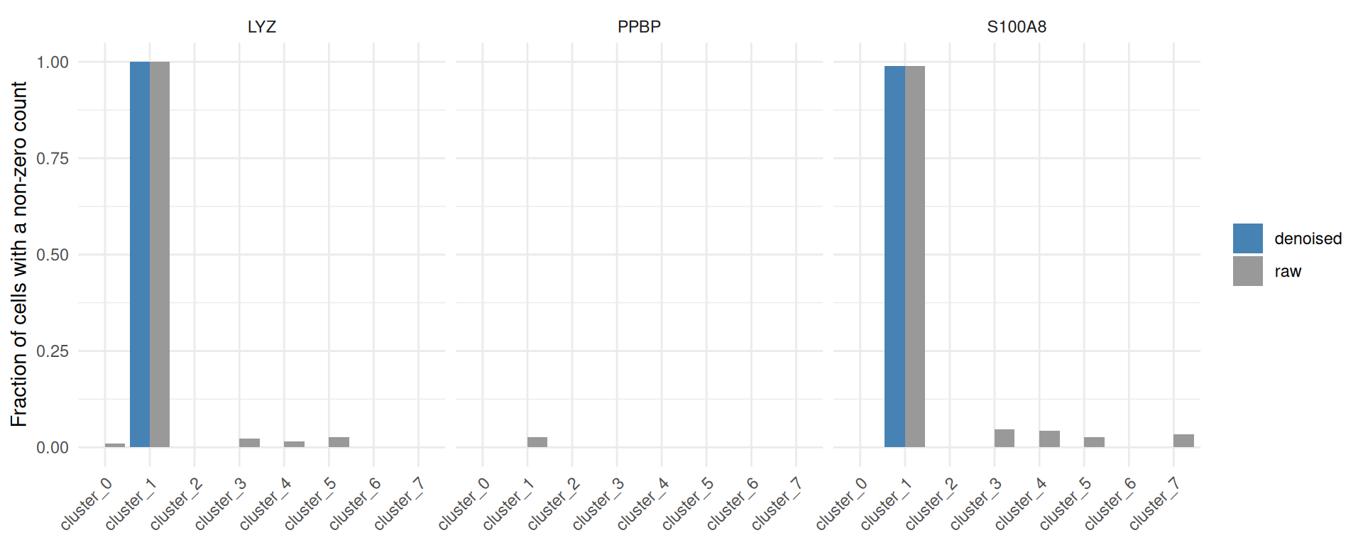
Cluster 1 is the monocytes and it keeps LYZ and S100A8 in essentially every cell. Everywhere else those genes were showing up in a few percent of barcodes before the sweep and are gone afterwards. PPBP does the same thing in reverse: platelet transcripts leaking into the monocytes disappear. The subtraction went after the right counts.
Reprocessing the clean counts
Feature selection and reduction were computed on contaminated counts, so they have to be redone. Drop the barcodes CellSweep says are mostly soup while you are at it.
clean_object <- set_cells_to_keep(
  clean_object,
  obs_clean[cellsweep_alpha <= 0.3, cell_id]
)

clean_object <- find_hvg_sc(clean_object, hvg_no = 2000L, .verbose = FALSE)

clean_object <- calculate_pca_sc(
  clean_object,
  no_pcs = 30L,
  sparse_svd = TRUE,
  .verbose = FALSE
)

clean_object <- find_neighbours_sc(
  clean_object,
  neighbours_params = params_sc_neighbours(
    knn = list(knn_method = "exhaustive")
  ),
  .verbose = FALSE
)

clean_object <- umap_sc(clean_object, .verbose = FALSE)

clean_object
#> Single cell experiment (Single Cells).
#>   No cells (original): 762
#>    To keep n: 755
#>   No genes: 36601
#>   HVG calculated: TRUE
#>   PCA calculated: TRUE
#>   Other embeddings: umap
#>   KNN generated: TRUE
#>   SNN generated: TRUE
#>   MAGIC imputed: none
#>   Residual model: none
#>   Stale artefacts: none
embedding_plot_sc(
  clean_object,
  embedding = "umap",
  colour_by = "cell_type",
  label_by = "cell_type",
  discrete = TRUE
)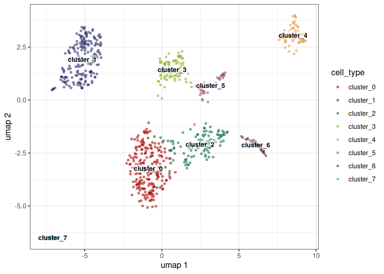
The clusters survive the sweep, which is what you want. CellSweep is not supposed to rearrange your populations, it is supposed to stop the space between them being filled with borrowed transcripts. If your structure falls apart after denoising, the labels you handed it were wrong.
Where this goes next
The obvious extension is multi-sample data, where the ambient profile is fitted per emulsion and sample_column starts earning its keep. A soup that differs between runs is a batch effect that no correction method will name for you, and having cellsweep_alpha and the per-sample profiles in hand is a much better starting point than pretending the contamination is uniform.
cellsweep_alpha is also worth keeping in the obs table after the fact. It is a QC metric in its own right, and a cluster with a suspiciously high median is usually debris rather than biology.
Clean up
unlink(tempdir_cellsweep, recursive = TRUE, force = TRUE)