
Bulk co-expression modules
2026-09-24
Intro
Bulk co-expression module detection tries to find groups of genes that vary together across samples. bixverse ships five approaches for this on a shared BulkCoExp class:
- CoReMo (Srivastava, et al.: hierarchical clustering on an RBF-transformed correlation matrix. Fast, deterministic, gives you signed modules and per-sample eigengenes.
- Graph-based Leiden (Barrio-Hernandez, et al.) — build a sparse affinity graph from correlations, then cluster with Leiden. Great when you want tunable resolution and hierarchical sub-clustering.
- ICA — independent component analysis with stability across random initialisations. Each component picks up an independent signal; the genes in the tails of a component’s loading distribution define its module.
- DGRDL (Pan, et al.) — dual graph-regularised dictionary learning. Sparse decomposition regularised by feature- and sample-side Laplacians.
-
NMF (HALS) — non-negative matrix factorisation with hierarchical alternating least squares. Non-negative loadings give a natural “parts-based” module interpretation and per-sample module activity. Comes in three flavours: one run, best-of-many restarts, or consensus across restarts (cNMF), which also hands you a way to choose
k.
One structural difference matters throughout. CoReMo and Leiden partition genes: one gene, one module. The three factorisation methods do not, and should not. A gene can load on several components, so get_modules() returns one row per (gene, component) pair for ICA, NMF and DGRDL, and genes in no component’s tail appear nowhere. params_module_membership() controls that thresholding. Do not assume gene is a unique key.
None of these is uniformly best. This vignette walks through all five on the same synthetic dataset with planted ground-truth modules, so you can see the inputs, the outputs, and how well each recovers the true structure.
Data
synthetic_bulk_cor_matrix() generates a bulk RNA-seq count matrix with heteroskedasticity plus a user-specified number of planted co-expression modules. Counts come from a negative binomial with a mean-dispersion trend, and a module is built by putting its genes on a shared latent factor.
params_synthetic_bulk_rnaseq() controls the whole thing. The parameter that matters most here is generator, which picks how loadings and factors are drawn:
-
hub_modular— LogNormal loadings on a Normal factor. Some genes end up far more connected than others, which is the WGCNA-style default and our starting point. -
modular— Beta(5, 2) loadings on a Normal factor. Homogeneous within-module correlation, no hubs. -
non_negative_factor— LogNormal loadings on a Gamma factor. The activity matrix is non-negative by construction, so NMF has a ground truth it can reach. -
non_gaussian_factor— LogNormal loadings on a Laplace factor. Non-Gaussian sources satisfy ICA identifiability.
We’ll start with hub_modular for the head-to-head, then come back to the generator choice at the end. It turns out to matter more than you’d guess.
synth_params <- params_synthetic_bulk_rnaseq(
  num_samples = 100L,
  num_genes = 1000L,
  module_sizes = c(100L, 100L, 100L),
  generator = "hub_modular",
  seed = 123L
)

synth <- synthetic_bulk_cor_matrix(synth_params)

truth <- synth$module_data
truth[membership > 0, .N, by = membership]
#>    membership     N
#>         <int> <int>
#> 1:          1   100
#> 2:          2   100
#> 3:          3   100
Three planted modules of 100 genes each. The remaining 700 genes are background: no loading, never a hub.
The ground truth comes back with the counts, so we can score a recovered module against what was actually simulated rather than eyeballing a heatmap. Per gene we get its module, its loading on that module’s factor, and whether it ranked as a hub:
Hubs are ranked on loading globally across all module genes rather than per module, so the counts per module don’t have to be equal. On top of that, $module_factors holds the latent factors themselves, one row per module:
dim(synth$module_factors)
#> [1]   3 100
That matrix is what a module eigengene, an ICA component or an NMF activity column is trying to recover, and we use it for a second scoring pass later on.
For the correlation-based methods we work in log-CPM space (negative values are fine); NMF needs non-negative input so we’ll build a separate object from the raw counts for it.
norm_counts <- rs_cpm(synth$counts, lib_size = NULL, log = TRUE, prior_count = 2)
raw_cpm <- rs_cpm(synth$counts, lib_size = NULL, log = FALSE, prior_count = 2)

data_log <- t(norm_counts)
data_raw <- t(raw_cpm)

meta_data <- data.table(sample_id = rownames(data_log))

coexp <- BulkCoExp(raw_data = data_log, meta_data = meta_data)
coexp <- preprocess_bulk_coexp(coexp, hvg = 0.5, .verbose = FALSE)
coexp
#> Bulk co-expression module class (BulkCoExp).
#>  Pre-processing done: TRUE.
#>   Number of HVG: 500.
Preprocessing keeps the top 50% of genes by MAD; 500 features carried through to the module-detection methods below. The BulkCoExp object mutates in place as each method runs, so we’ll make copies for each branch.
Method 1: CoReMo
CoReMo shrinks weak correlations via an RBF, hierarchically clusters the result, and picks the cut that maximises the within-module weighted median R². The epsilon parameter controls how aggressively the RBF suppresses weak correlations — you usually tune it against a scale-free topology fit.
coexp_coremo <- cor_module_processing(
  coexp,
  cor_method = "spearman",
  .verbose = TRUE
)
#> Using Spearman correlations.

# show correlation structure
coexp_coremo@processed_data$correlation_res$get_data_table() %$% hist(sim)
#> Generating data.table format of the symmetric matrix.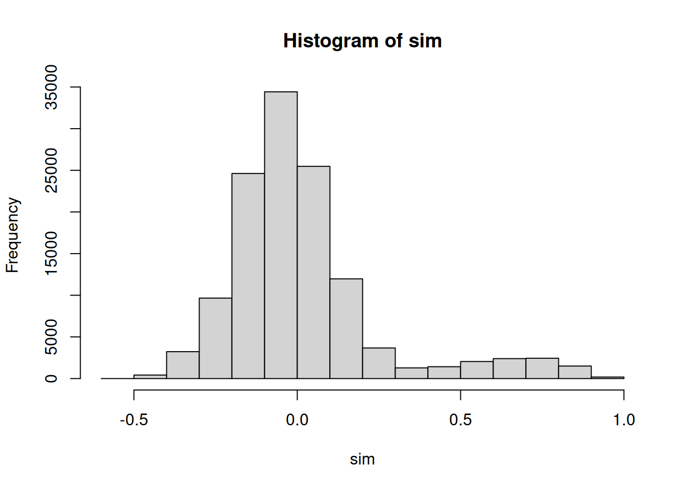
coexp_coremo <- cor_module_check_epsilon(
  coexp_coremo,
  rbf_func = "gaussian",
  .verbose = TRUE
)
#> Testing 21 epsilons.

plot_epsilon_res(coexp_coremo)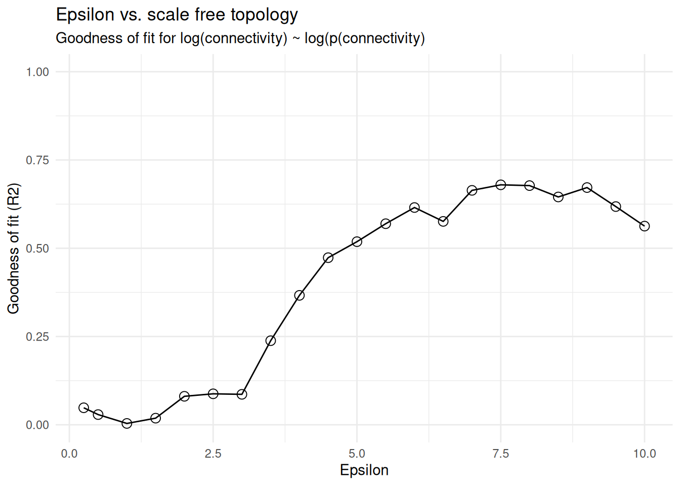
epsilon_sf <- get_epsilon_res(coexp_coremo)[r2_vals == max(r2_vals), epsilon][1]
epsilon_sf
#> [1] 7.5
Here is a wrinkle worth knowing about, and one the ground truth lets us actually diagnose. The scale-free R² criterion picks a high epsilon, but epsilon controls how aggressively the RBF suppresses weak correlations, so a high value throws genes out of modules entirely. Counting how many of the 500 features survive into a module tells the story:
epsilon_scan <- rbindlist(lapply(c(1, 2, 3, 4, 6, epsilon_sf), \(eps) {
  fitted <- coexp_coremo %>%
    cor_module_coremo_clustering(
      coremo_params = params_coremo(epsilon = eps, rbf_func = "gaussian"),
      .verbose = FALSE
    ) %>%
    cor_module_coremo_stability(.verbose = FALSE) %>%
    cor_module_coremo_cor_sign(.verbose = FALSE)

  mods <- get_outputs(fitted)$final_modules
  data.table(
    epsilon = eps,
    n_modules = uniqueN(mods$cluster_id),
    genes_assigned = nrow(mods)
  )
}))

epsilon_scan
#>    epsilon n_modules genes_assigned
#>      <num>     <int>          <int>
#> 1:     1.0         4            254
#> 2:     2.0         5            253
#> 3:     3.0         4            207
#> 4:     4.0         4            167
#> 5:     6.0         2             55
#> 6:     7.5         4            103
The scale-free fit and “keep as many real module genes as possible” pull in opposite directions on this data. We go with a low epsilon deliberately, because the planted modules are what we are trying to find:
coremo_params <- params_coremo(epsilon = 2, rbf_func = "gaussian")

coexp_coremo <- cor_module_coremo_clustering(
  coexp_coremo,
  coremo_params = coremo_params,
  .verbose = TRUE
)
#> Generating the full matrix format of the symmetric matrix.
#> Generating the hierarchical clustering.
#> Identifying optimal number of cuts.
#> Finalising CoReMo clusters.
coexp_coremo <- cor_module_coremo_stability(coexp_coremo, .verbose = FALSE)
coexp_coremo <- cor_module_coremo_cor_sign(coexp_coremo, .verbose = FALSE)
coexp_coremo <- cor_module_coremo_eigengene(coexp_coremo, .verbose = FALSE)

coremo_modules <- get_outputs(coexp_coremo)$final_modules
coremo_modules[, .N, by = cluster_id]
#>    cluster_id     N
#>        <char> <int>
#> 1:      2_pos    79
#> 2:      1_pos    83
#> 3:      3_pos    63
#> 4:      5_pos    27
#> 5:      5_neg     1
Each module has a sign suffix (_pos / _neg) reflecting whether the member genes are positively or negatively correlated with the module eigengene, and a per-gene stability score from the leave-one-out resampling. Since the generator draws strictly positive loadings, essentially everything lands in a _pos module; the odd _neg singleton is an anti-correlated background gene getting split off, which is correct behaviour.
Method 2: Graph-based Leiden
The Leiden branch keeps the same RBF-based affinity but treats the sparse non-zero pattern as an igraph. Modularity is optimised over a Leiden resolution grid; large communities can be sub-clustered recursively.
coexp_leiden <- cor_module_processing(
  coexp,
  cor_method = "spearman",
  .verbose = TRUE
)
#> Using Spearman correlations.

coexp_leiden <- cor_module_check_epsilon(
  coexp_leiden,
  rbf_func = "bump",
  .verbose = TRUE
)
#> Testing 21 epsilons.

plot_epsilon_res(coexp_leiden)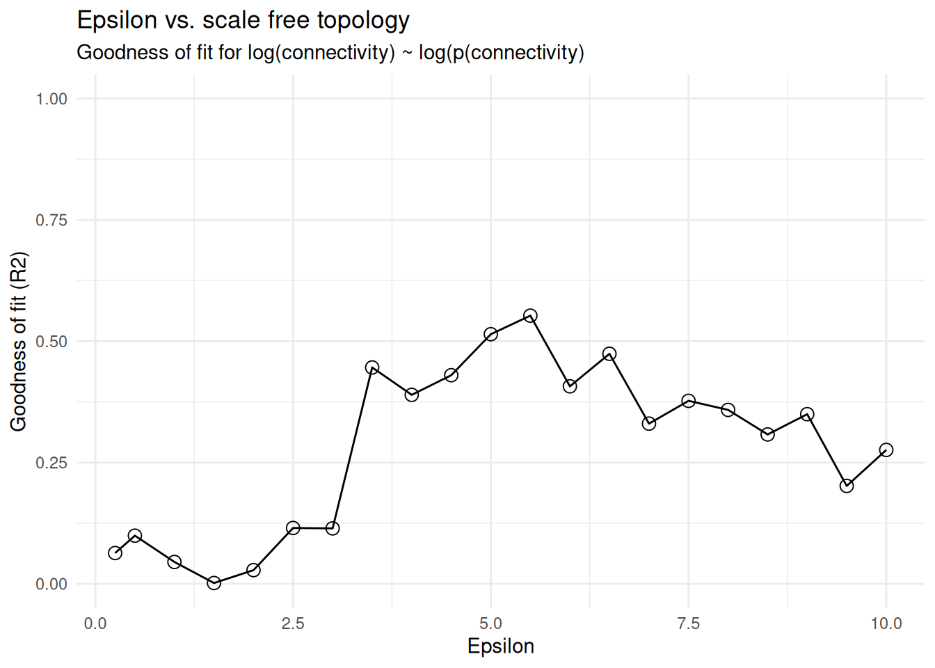
graph_params <- params_cor_graph(
  epsilon = 2
)

coexp_leiden <- cor_module_graph_check_res(
  coexp_leiden,
  resolution_params = params_graph_resolution(),
  graph_params = graph_params,
  parallel = FALSE,
  .verbose = TRUE
)
#> Generating data.table format of the symmetric matrix.
#> Generating correlation-based graph with 8567 edges.
#> Iterating through 15 resolutions
#> Using sequential computation.

plot_resolution_res(coexp_leiden)
#> Key: <resolution>
#>    resolution no_clusters modularity good_clusters avg_size max_size
#>         <num>       <int>      <num>         <int>    <num>    <int>
#> 1:  0.1000000           3  0.6559388             3 83.66667       88
#> 2:  0.1389495           3  0.6559388             3 83.66667       88
#> 3:  0.1930698           3  0.6559388             3 83.66667       88
#> 4:  0.2682696           3  0.6559388             3 83.66667       88
#> 5:  0.3727594           3  0.6559388             3 83.66667       88
#> 6:  0.5179475           3  0.6559388             3 83.66667       88
#> Warning in sqrt(x): NaNs produced
#> Warning: Removed 3 rows containing missing values or values outside the scale range
#> (`geom_point()`).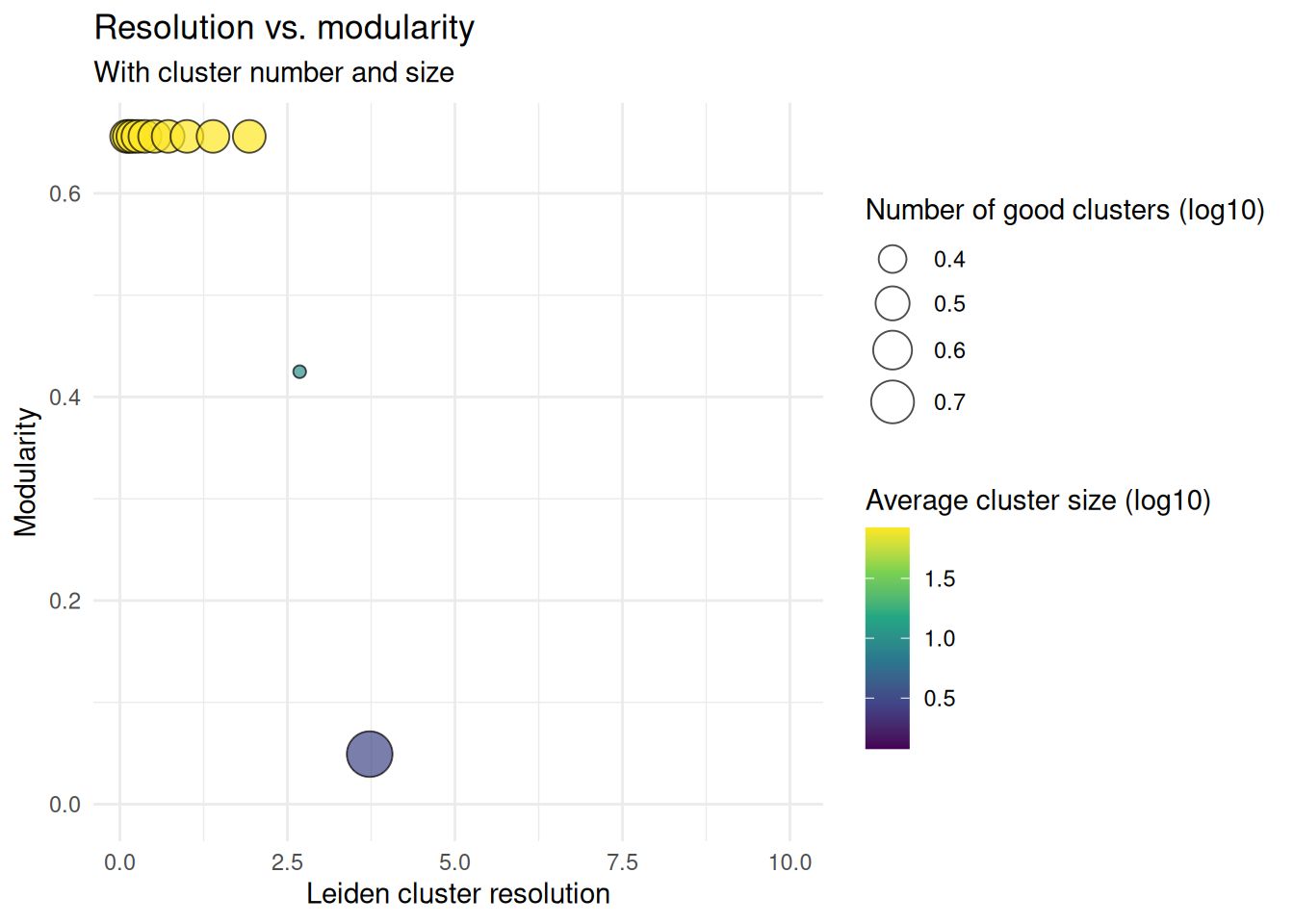
coexp_leiden <- cor_module_graph_final_modules(
  coexp_leiden,
  min_size = 10L,
  max_size = 500L,
  subclustering = TRUE,
  .graph_params = graph_params,
  .verbose = FALSE
)

leiden_modules <- get_modules(get_results(coexp_leiden))
leiden_modules[, .N, by = module_id]
#>    module_id     N
#>       <char> <int>
#> 1: cluster_1    84
#> 2: cluster_2    79
#> 3: cluster_3    88
Method 3: ICA
ICA whitens the data, then finds independent components across many random initialisations. The stability across restarts, the fraction of converged runs, and the mutual information between components combine into a combined_score: the loess inflection point of this score against the number of components gives you an “optimal” ncomp. (Please explore your data and see how it looks…)
coexp_ica <- ica_processing(coexp, fast_svd = TRUE, .verbose = FALSE)

# A dense enough grid that the loess in ica_optimal_ncomp() has something to
# fit. On a handful of points it gives up and warns instead.
ncomp_params <- params_ica_ncomp(max_no_comp = 30L, steps = 2L)
iter_params <- params_ica_randomisation(
  cross_validate = FALSE,
  random_init = 20L
)

coexp_ica <- ica_evaluate_comp(
  coexp_ica,
  ica_type = "logcosh",
  iter_params = iter_params,
  ncomp_params = ncomp_params,
  .verbose = FALSE
)

coexp_ica <- ica_optimal_ncomp(
  coexp_ica,
  span = 0.4,
  show_plot = FALSE,
  .verbose = FALSE
)
coexp_ica <- ica_stabilised_results(
  coexp_ica,
  iter_params = iter_params,
  .verbose = FALSE
)

ica_res <- get_results(coexp_ica)
ica_gene_loadings <- get_factors(ica_res, which = "gene_loadings")
dim(ica_gene_loadings)
#> [1] 500   5
gene_loadings is the genes x k matrix (transposed from the raw ICA S convention of k x genes). Module membership keeps the tails of each component, so a gene may appear more than once and many genes not at all:
ica_modules <- get_modules(ica_res)
ica_modules[, .N, by = module_id][order(-N)]
#>    module_id     N
#>       <char> <int>
#> 1:      IC_5    90
#> 2:      IC_1    58
#> 3:      IC_4    48
#> 4:      IC_2    38
#> 5:      IC_3    35

# Sparse and overlapping, which is the whole point of a factorisation.
data.table(
  rows = nrow(ica_modules),
  unique_genes = uniqueN(ica_modules$gene),
  in_multiple_modules = ica_modules[, .N, by = gene][N > 1, .N]
)
#>     rows unique_genes in_multiple_modules
#>    <int>        <int>               <int>
#> 1:   269          151                  63
Method 4: DGRDL
DGRDL learns a sparse dictionary of features constrained by a k-nearest- neighbour Laplacian on both the feature and the sample side. The grid search helps pick dict_size and k_neighbours before the final fit.
Unlike the other four, DGRDL needs centred input. Handed unscaled log-CPM it spends its dictionary explaining the per-gene mean offset instead of the covariance: atoms come out as near-duplicates of each other, and the loadings become a large constant plus noise. So we build a scaled object for it.
coexp_dgrdl <- BulkCoExp(raw_data = data_log, meta_data = meta_data) %>%
  preprocess_bulk_coexp(
    hvg = 0.5,
    scaling = TRUE,
    scaling_type = "normal",
    .verbose = FALSE
  )

coexp_dgrdl <- dgrdl_grid_search(
  coexp_dgrdl,
  neighbours_vec = c(5L, 10L),
  dict_size_vec = c(4L, 6L),
  seed_vec = c(1L, 2L),
  dgrdl_params = params_dgrdl(),
  .verbose = TRUE
)
#> A total of 8 parameters will be tested in a grid search for DGRDL.

grid_res <- get_grid_search_res(coexp_dgrdl)
setorder(grid_res, reconstruction_errs)
head(grid_res)
#>     seed dict_size k_neighbours reconstruction_errs feature_laplacian_objective
#>    <num>     <num>        <num>               <num>                       <num>
#> 1:     1         4            5             3157249                    98876.33
#> 2:     1         4           10             3157249                   196361.51
#> 3:     2         4            5             3157305                    98864.44
#> 4:     2         4           10             3157305                   196338.53
#> 5:     2         6            5             4831244                   149155.31
#> 6:     2         6           10             4831245                   294733.43
#>    sample_laplacian_objective
#>                         <num>
#> 1:                   1.700723
#> 2:                   3.085984
#> 3:                   1.700597
#> 4:                   3.085838
#> 5:                   2.602797
#> 6:                   4.898748
Pick the top row and fit the final DGRDL model:
top <- grid_res[1L]

dgrdl_params_final <- params_dgrdl(
  dict_size = as.integer(top$dict_size),
  k_neighbours = as.integer(top$k_neighbours)
)

coexp_dgrdl <- dgrdl_result(
  coexp_dgrdl,
  dgrdl_params = dgrdl_params_final,
  seed = as.integer(top$seed),
  .verbose = FALSE
)

dgrdl_res <- get_results(coexp_dgrdl)
dim(get_factors(dgrdl_res, which = "dictionary"))
#> [1] 100   4
dim(get_factors(dgrdl_res, which = "loadings"))
#> [1]   4 500
get_modules() keeps the tails of each dictionary atom, so a gene active in several atoms shows up in several modules:
dgrdl_modules <- get_modules(dgrdl_res)
dgrdl_modules[, .N, by = module_id][order(-N)]
#>    module_id     N
#>       <char> <int>
#> 1:    dict_1    53
#> 2:    dict_4    52
#> 3:    dict_2    49
#> 4:    dict_3    32
Method 5: NMF (HALS)
NMF needs non-negative input, so we build a fresh BulkCoExp from CPM (without the log transform). The single-run version is deterministic given NNDSVD initialisation; the stabilised version runs multiple random restarts and returns the run with the lowest reconstruction loss.
coexp_nmf <- BulkCoExp(raw_data = data_raw, meta_data = meta_data)
coexp_nmf <- preprocess_bulk_coexp(coexp_nmf, hvg = 0.5, .verbose = FALSE)

coexp_nmf <- nmf_bulk(
  coexp_nmf,
  k = 4L,
  preprocessing = "none",
  nmf_hals_params = params_nmf_hals(max_iter = 300L, tol = 1e-4),
  seed = 42L,
  .verbose = FALSE
)

nmf_modules <- get_nmf_modules(coexp_nmf)
nmf_modules[, .N, by = module_id]
#>    module_id     N
#>       <char> <int>
#> 1:   comp_01     3
#> 2:   comp_02    68
#> 3:   comp_03    67
#> 4:   comp_04    71
get_nmf_gene_loadings() gives the features x k matrix, and get_nmf_sample_activity() gives the samples x k matrix. A quick heatmap of gene loadings shows the parts-based decomposition:
loadings <- get_nmf_gene_loadings(coexp_nmf)

top_genes <- unique(unlist(lapply(seq_len(ncol(loadings)), \(j) {
  names(sort(loadings[, j], decreasing = TRUE))[1:40]
})))

heat_dt <- as.data.table(
  loadings[top_genes, , drop = FALSE],
  keep.rownames = "gene"
)
heat_long <- melt(
  heat_dt,
  id.vars = "gene",
  variable.name = "component",
  value.name = "loading"
)

ggplot(heat_long, aes(component, gene, fill = loading)) +
  geom_tile() +
  scale_fill_viridis_c() +
  theme_minimal() +
  theme(axis.text.y = element_blank(), axis.ticks.y = element_blank())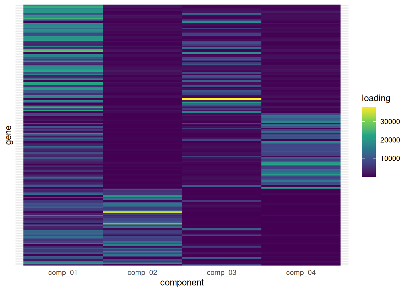
For a more robust fit, stabilised_nmf_bulk() runs several restarts and returns per-run losses via get_nmf_stability().
coexp_nmf_stab <- stabilised_nmf_bulk(
  coexp_nmf,
  k = 4L,
  n_runs = 5L,
  preprocessing = "none",
  nmf_hals_params = params_nmf_hals(max_iter = 200L, tol = 1e-3),
  seed = 7L,
  .verbose = FALSE
)

stab <- get_nmf_stability(coexp_nmf_stab)
stab
#> $losses
#> [1] 6901265228 6885273325 6903864049 6878840096 6887485166
#>
#> $converged
#> [1] TRUE TRUE TRUE TRUE TRUE
#>
#> $best_idx
#> [1] 4
Consensus NMF
stabilised_nmf_bulk() picks the restart with the lowest loss, which tells you nothing about whether that restart is reproducible. Consensus NMF asks the better question: pool the components of every restart, throw away the ones that sit on their own, cluster what is left into k groups, and take the median of each group as the answer. What survives is the structure the restarts agree on. That agreement gets a number, the mean silhouette of those clusters, and it is the honest way to judge whether k is right.
Which brings us to picking k. nmf_k_sweep_bulk() runs the whole thing across a range and reports stability against reconstruction error, no factors kept, so it stays cheap.
k_sweep <- nmf_k_sweep_bulk(
  coexp_nmf,
  k_range = 2:8,
  n_runs = 10L,
  preprocessing = "none",
  nmf_hals_params = params_nmf_hals(max_iter = 200L, tol = 1e-3),
  nmf_consensus_params = params_nmf_consensus(density_threshold = 2),
  seed = 42L,
  .verbose = TRUE
)

k_sweep
#> NmfKSweepResult (consensus NMF k sweep)
#>   Source class:     BulkCoExp
#>   k range:          2 to 8
#>   No runs per k:    10
#>   Most stable k:    4 (stability = 0.9752)
#>
#>        k stability best_error median_error consensus_failed n_dropped
#>    <int>     <num>      <num>        <num>           <lgcl>     <int>
#> 1:     2 0.7546717 0.13438072   0.13449627            FALSE         0
#> 2:     3 0.7082610 0.09671029   0.09806779            FALSE         0
#> 3:     4 0.9751885 0.06291160   0.06299967            FALSE         0
#> 4:     5 0.8993866 0.05916342   0.06091455            FALSE         0
#> 5:     6 0.7649848 0.05695935   0.05906541            FALSE         0
#> 6:     7 0.7087608 0.05512725   0.05638576            FALSE         0
#> 7:     8 0.6015507 0.05385696   0.05448819            FALSE         0
#>    n_empty_clusters n_converged
#>               <int>       <int>
#> 1:                0          10
#> 2:                0          10
#> 3:                0          10
#> 4:                0          10
#> 5:                0          10
#> 6:                0          10
#> 7:                0          10
plot(k_sweep)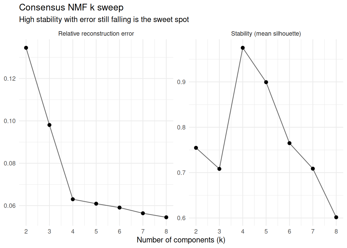
Error falls monotonically with k, so on its own it would push you to the largest k you can afford. Stability is the counterweight. You want the last k before it drops off, where the error curve is still coming down.
Note
density_threshold = 2switches the outlier filter off, because cosine distance cannot exceed 2. With the filter live, components whose neighbours sit far away get dropped, and if that leaves fewer thankof them the fit errors rather than handing back something degenerate. That is the right behaviour on real data, but with only 10 restarts on a small synthetic matrix it fires more often than it should. Plotlocal_densityfromget_nmf_stability()to pick a real threshold for your data.
Now fit at the chosen k:
coexp_nmf_consensus <- consensus_nmf_bulk(
  coexp_nmf,
  k = 4L,
  n_runs = 10L,
  preprocessing = "none",
  nmf_hals_params = params_nmf_hals(max_iter = 300L, tol = 1e-4),
  nmf_consensus_params = params_nmf_consensus(density_threshold = 2),
  seed = 42L,
  .verbose = FALSE
)

consensus_stab <- get_nmf_stability(coexp_nmf_consensus)
consensus_stab$stability
#> [1] 0.988677
consensus_stab$cluster_sizes
#>    cluster     n
#>      <int> <int>
#> 1:       1    10
#> 2:       2    10
#> 3:       3    10
#> 4:       4    10
The per-component table shows where every restart’s components ended up. component_id uses the same run_XX.comp_YY naming as the w_all columns of a stabilised fit, so at matching k and n_runs the two line up directly.
head(consensus_stab$clusters)
#>      component_id   run component pooled_idx cluster local_density silhouette
#>            <char> <int>     <int>      <int>   <int>         <num>      <num>
#> 1: run_01.comp_01     1         1          1       3  5.220118e-06  0.9999714
#> 2: run_01.comp_02     1         2          2       4  9.438175e-03  0.9763555
#> 3: run_01.comp_03     1         3          3       1  7.572240e-03  0.9526643
#> 4: run_01.comp_04     1         4          4       2  1.848401e-04  0.9952859
#> 5: run_02.comp_01     2         1          5       2  5.203952e-05  0.9968476
#> 6: run_02.comp_02     2         2          6       3  6.306892e-07  0.9999903
#>      kept
#>    <lgcl>
#> 1:   TRUE
#> 2:   TRUE
#> 3:   TRUE
#> 4:   TRUE
#> 5:   TRUE
#> 6:   TRUE
nmf_consensus_modules <- get_nmf_modules(coexp_nmf_consensus)
nmf_consensus_modules[, .N, by = module_id]
#>    module_id     N
#>       <char> <int>
#> 1:   comp_01    57
#> 2:   comp_02    66
#> 3:   comp_03     3
#> 4:   comp_04    54
Recovery of planted modules
With ground truth in hand we can quantify how well each method recovered the three planted modules. For each method we compute the best-matching planted module per detected cluster (max Jaccard), then take the mean Jaccard across the three planted modules…. A simple “recall” score.
# assignments: data.table with columns `gene` and `module_id`.
# Returns one score per planted module: the best Jaccard any detected cluster
# manages against it.
best_jaccard_vs <- function(assignments, truth_dt) {
  planted <- split(truth_dt$gene, truth_dt$membership)
  planted <- planted[names(planted) != "0"]
  detected <- split(assignments$gene, assignments$module_id)
  purrr::map_dbl(planted, \(p) {
    max(purrr::map_dbl(detected, \(d) {
      length(intersect(p, d)) / length(union(p, d))
    }))
  })
}

recovery <- data.table(
  method = c("CoReMo", "Leiden", "ICA", "DGRDL", "NMF", "Consensus NMF"),
  score = c(
    mean(best_jaccard_vs(
      coremo_modules[, .(gene, module_id = cluster_id)],
      truth
    )),
    mean(best_jaccard_vs(leiden_modules, truth)),
    mean(best_jaccard_vs(ica_modules, truth)),
    mean(best_jaccard_vs(dgrdl_modules, truth)),
    mean(best_jaccard_vs(nmf_modules, truth)),
    mean(best_jaccard_vs(nmf_consensus_modules, truth))
  )
)

setorder(recovery, -score)
recovery
#>           method     score
#>           <char>     <num>
#> 1:        Leiden 0.8366667
#> 2:        CoReMo 0.7500000
#> 3:           NMF 0.6811551
#> 4: Consensus NMF 0.5900000
#> 5:           ICA 0.4809684
#> 6:         DGRDL 0.1505952
ggplot(recovery, aes(x = reorder(method, score), y = score)) +
  geom_col(fill = "steelblue") +
  coord_flip() +
  ylim(0, 1) +
  theme_minimal() +
  xlab("") +
  ylab("Mean best Jaccard vs. planted modules")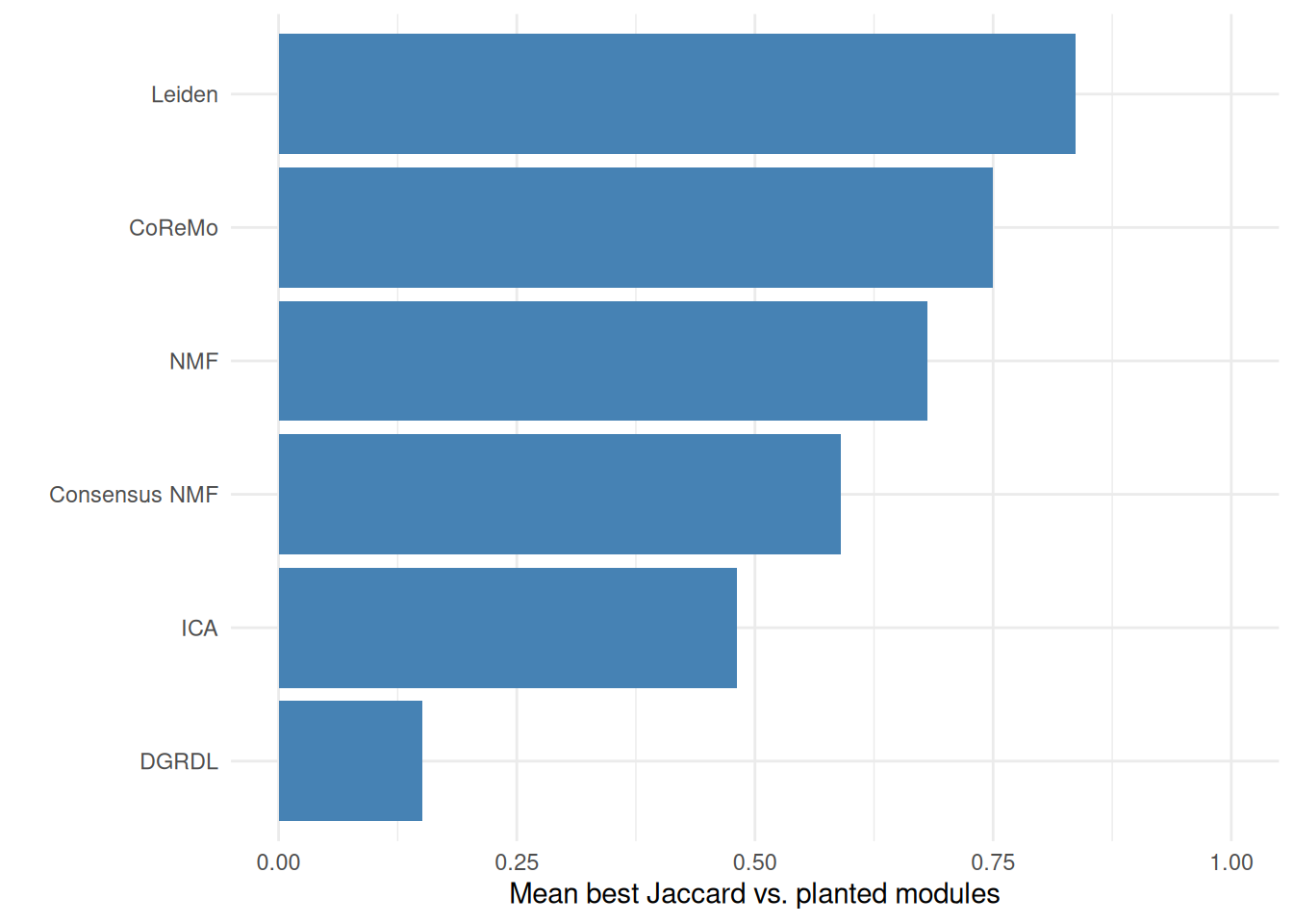
Worth being blunt about one result there: consensus NMF scores below plain NMF. That is not a bug, and it is not an argument against consensus NMF. Two things are going on. This data was generated with hub_modular, a Normal latent factor, so there is no non-negative ground truth for NMF to reach in the first place, and both NMF variants are fighting the data. On top of that, consensus optimises for reproducibility, not recall: the median across restarts is deliberately conservative, and the components it keeps are the ones every restart found rather than the ones that happen to match a planted module best on one lucky seed. A recall number on simulated data rewards the lucky seed. Real data does not.
Scoring against the latent factors
Jaccard on gene sets only asks whether a method found the right genes. The latent factors let us ask a sharper question: did it recover the right signal? For CoReMo we can correlate each per-sample eigengene against the factor the module was actually built on.
# activity: samples x k matrix of per-sample scores (eigengenes, ICA sample
# activity, NMF sample activity). Returns one score per true factor: the best
# absolute correlation any recovered column manages against it.
#
# Index the factor matrix by rownames(activity), not by column position: these
# per-sample matrices come back in lexicographic sample order (sample_1,
# sample_10, sample_100, ...) while module_factors is in numeric order. Line them
# up positionally and you get correlations near zero for no good reason.
best_factor_cor <- function(activity, module_factors) {
  purrr::map_dbl(seq_len(nrow(module_factors)), \(k) {
    true_factor <- module_factors[k, rownames(activity)]
    max(apply(activity, 2, \(a) {
      abs(cor(a, true_factor, method = "spearman"))
    }))
  })
}

eigengenes <- get_factors(get_results(coexp_coremo))$module_eigengenes

data.table(
  module = rownames(synth$module_factors),
  best_abs_cor = round(best_factor_cor(eigengenes, synth$module_factors), 3)
)
#>      module best_abs_cor
#>      <char>        <num>
#> 1: module_1        0.984
#> 2: module_2        0.984
#> 3: module_3        0.987
Those sit far higher than the Jaccard scores, and the gap is the interesting part: CoReMo reconstructs the module’s signal almost exactly even where it disagrees with the planted gene list at the edges. If what you care about is a per-sample module score to regress against a phenotype, the eigengene is doing its job well before the gene membership is perfect.
Does the generator matter?
A lot, and the answer depends on what you measure. non_negative_factor advertises itself as NMF-friendly and non_gaussian_factor as ICA-friendly, so the obvious guess is that each method wins on its matched generator. We score two ways to see whether that holds:
- Jaccard, as above: a hard partition of genes into modules, compared against the planted gene sets.
- Factor recovery: the best absolute correlation any recovered per-sample activity column achieves against a true latent factor.
The distinction matters because “ICA-friendly” is a claim about identifiability of the factorisation, that is, recovering the sources up to permutation and scaling. It says nothing about whether assigning each gene to its strongest-loading component reproduces a planted block. Three methods rather than five here, to keep the render time honest: Leiden and DGRDL both carry a parameter search on top.
run_methods <- function(generator) {
  params <- params_synthetic_bulk_rnaseq(
    num_samples = 100L,
    num_genes = 1000L,
    module_sizes = c(100L, 100L, 100L),
    generator = generator,
    seed = 123L
  )
  synth_g <- synthetic_bulk_cor_matrix(params)
  meta_g <- data.table(sample_id = colnames(synth_g$counts))

  log_obj <- BulkCoExp(
    raw_data = t(rs_cpm(
      synth_g$counts,
      lib_size = NULL,
      log = TRUE,
      prior_count = 2
    )),
    meta_data = meta_g
  ) %>%
    preprocess_bulk_coexp(hvg = 0.5, .verbose = FALSE)

  raw_obj <- BulkCoExp(
    raw_data = t(rs_cpm(
      synth_g$counts,
      lib_size = NULL,
      log = FALSE,
      prior_count = 2
    )),
    meta_data = meta_g
  ) %>%
    preprocess_bulk_coexp(hvg = 0.5, .verbose = FALSE)

  coremo_g <- log_obj %>%
    cor_module_processing(cor_method = "spearman", .verbose = FALSE) %>%
    cor_module_coremo_clustering(
      coremo_params = params_coremo(epsilon = 2),
      .verbose = FALSE
    ) %>%
    cor_module_coremo_stability(.verbose = FALSE) %>%
    cor_module_coremo_cor_sign(.verbose = FALSE) %>%
    cor_module_coremo_eigengene(.verbose = FALSE)

  ica_g <- log_obj %>%
    ica_processing(fast_svd = TRUE, .verbose = FALSE) %>%
    ica_evaluate_comp(
      ica_type = "logcosh",
      iter_params = iter_params,
      ncomp_params = ncomp_params,
      .verbose = FALSE
    ) %>%
    ica_optimal_ncomp(span = 0.4, show_plot = FALSE, .verbose = FALSE) %>%
    ica_stabilised_results(iter_params = iter_params, .verbose = FALSE)

  nmf_g <- nmf_bulk(
    raw_obj,
    k = 4L,
    preprocessing = "none",
    seed = 42L,
    .verbose = FALSE
  )

  truth_g <- synth_g$module_data
  coremo_mods <- get_outputs(coremo_g)$final_modules
  coremo_res_g <- get_results(coremo_g)
  ica_res_g <- get_results(ica_g)

  jacc <- \(assign) round(mean(best_jaccard_vs(assign, truth_g)), 3)
  fcor <- \(act) round(mean(best_factor_cor(act, synth_g$module_factors)), 3)

  data.table(
    generator = generator,
    metric = c("jaccard", "factor_cor"),
    CoReMo = c(
      jacc(coremo_mods[, .(gene, module_id = cluster_id)]),
      fcor(get_factors(coremo_res_g)$module_eigengenes)
    ),
    ICA = c(
      jacc(get_modules(ica_res_g)),
      fcor(get_factors(ica_res_g, which = "sample_activity"))
    ),
    NMF = c(
      jacc(get_nmf_modules(nmf_g)),
      fcor(get_nmf_sample_activity(nmf_g))
    )
  )
}

grid_res <- rbindlist(lapply(
  c("hub_modular", "modular", "non_negative_factor", "non_gaussian_factor"),
  run_methods
))

grid_res
#>              generator     metric CoReMo   ICA   NMF
#>                 <char>     <char>  <num> <num> <num>
#> 1:         hub_modular    jaccard  0.750 0.481 0.681
#> 2:         hub_modular factor_cor  0.985 0.523 0.988
#> 3:             modular    jaccard  0.790 0.200 0.690
#> 4:             modular factor_cor  0.983 0.635 0.986
#> 5: non_negative_factor    jaccard  0.563 0.495 0.486
#> 6: non_negative_factor factor_cor  0.959 0.440 0.966
#> 7: non_gaussian_factor    jaccard  0.617 0.526 0.596
#> 8: non_gaussian_factor factor_cor  0.978 0.567 0.979
grid_long <- melt(
  grid_res,
  id.vars = c("generator", "metric"),
  variable.name = "method",
  value.name = "score"
)

ggplot(grid_long, aes(x = generator, y = method, fill = score)) +
  geom_tile() +
  geom_text(aes(label = sprintf("%.2f", score)), colour = "white") +
  scale_fill_viridis_c(limits = c(0, 1)) +
  facet_wrap(~metric) +
  theme_minimal() +
  theme(axis.text.x = element_text(angle = 30, hjust = 1)) +
  xlab("") +
  ylab("")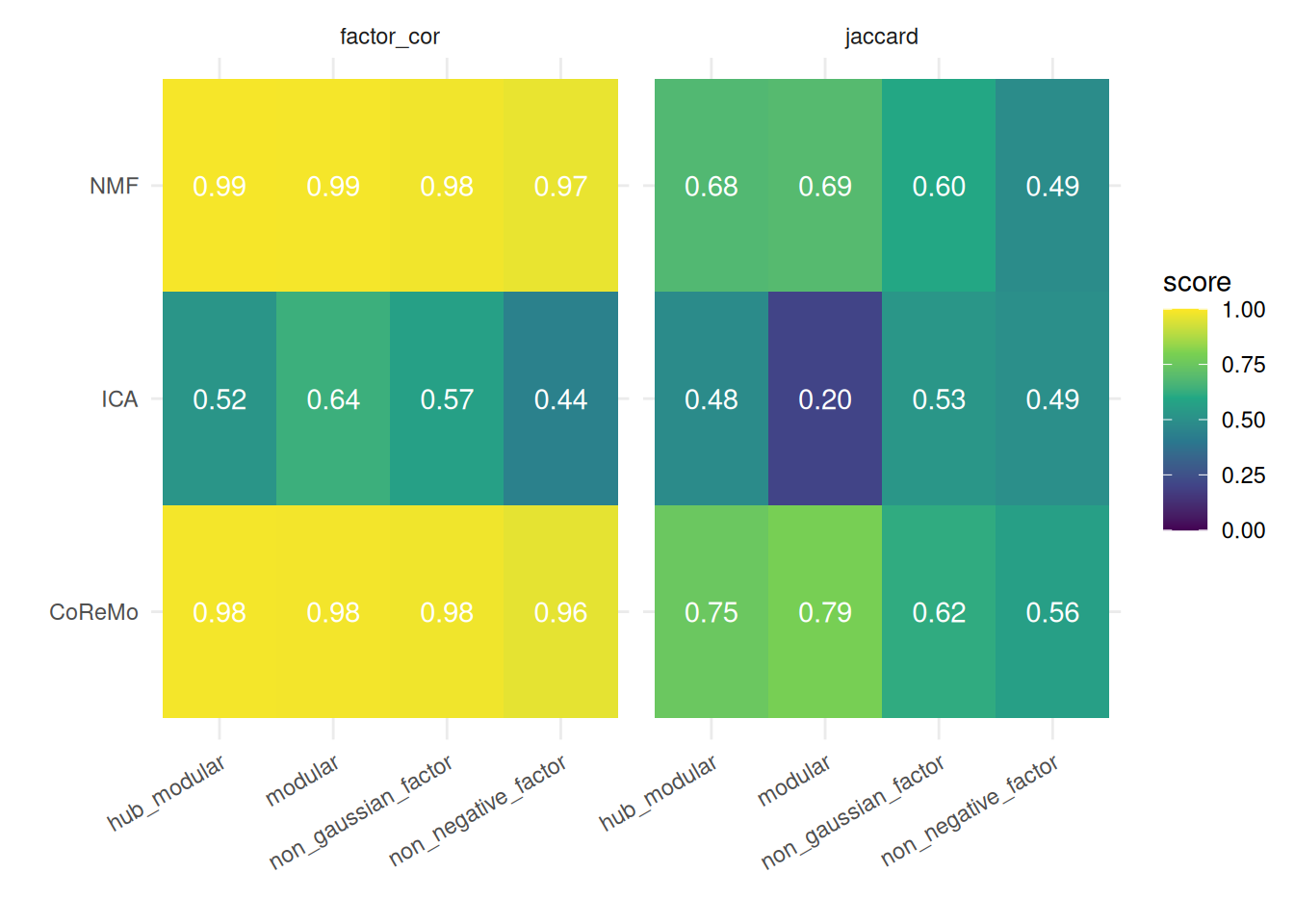
Two things to read out of that.
ICA’s factor recovery is best on non_gaussian_factor, exactly as advertised. The Laplace-factor generator is the one built for ICA and it wins on the metric identifiability is actually about. NMF’s factor recovery sits above 0.96 on all four, so that metric does not discriminate for NMF at all: it recovers per-sample activity almost perfectly regardless.
ICA’s Jaccard on modular collapses, and the reason is instructive. Membership for the factorisation methods comes from keeping the tails of each component’s loading distribution, which quietly assumes there is a tail. That assumption depends entirely on how the loadings were drawn:
excess_kurtosis <- function(x) {
  centred <- x - mean(x)
  mean(centred^4) / (mean(centred^2)^2) - 3
}

rbindlist(lapply(
  c("hub_modular", "modular", "non_negative_factor", "non_gaussian_factor"),
  \(gen) {
    synth_g <- synthetic_bulk_cor_matrix(params_synthetic_bulk_rnaseq(
      num_samples = 100L,
      num_genes = 1000L,
      module_sizes = c(100L, 100L, 100L),
      generator = gen,
      seed = 123L
    ))
    loadings_g <- synth_g$module_data[membership > 0, loading]
    data.table(
      generator = gen,
      loading_cv = round(sd(loadings_g) / mean(loadings_g), 2),
      loading_kurtosis = round(excess_kurtosis(loadings_g), 2)
    )
  }
))
#>              generator loading_cv loading_kurtosis
#>                 <char>      <num>            <num>
#> 1:         hub_modular       0.80             9.79
#> 2:             modular       0.23            -0.15
#> 3: non_negative_factor       0.75             8.83
#> 4: non_gaussian_factor       0.81             9.86
modular draws Beta(5, 2), so module-gene loadings have a coefficient of variation around 0.23: a tight, homogeneous block. Push that through ICA and the resulting component loadings come out sub-Gaussian, with negative excess kurtosis, and essentially nothing clears abs(z) > 3. There is no tail, so a tail-based rule finds nothing and Jaccard bottoms out. The three LogNormal generators have a loading CV around 0.8 and produce strongly leptokurtic components, where the rule works as designed.
So modular is a good benchmark for correlation and graph clustering, which threshold a similarity, and a poor one for matrix factorisation, which thresholds a loading tail. That is a property of the generator and metric pairing, not a verdict on any method.
Two practical lessons. Pick the generator that matches the property you are measuring and state which one you used, because a method that looks twice as good as another may simply have been handed a friendlier dataset. And if a factorisation returns almost no modules, check the kurtosis of its loadings before blaming the algorithm: you may just need a different cutoff in params_module_membership(), or a generator whose loadings have a tail at all.
Wrap-up
Different methods suit different questions:
- CoReMo if you want signed modules with per-sample eigengenes and a fast, deterministic pipeline. Solid default for standard bulk data.
- Graph-based Leiden if you want tunable resolution or hierarchical sub-clustering. Handles very heterogeneous module sizes better than CoReMo.
- ICA if you want components that decompose independent, potentially overlapping biological signals. Interpretation is per-component, not per-gene.
-
DGRDL if you want a sparse dictionary regularised by feature and sample neighbour graphs. Sparsity is a tunable constraint, not a byproduct. It comes last on recovery here, and note that
dgrdl_grid_search()ranks by reconstruction error, which is not the same objective as recovering planted modules. Remember to centre the input! - NMF if you want non-negative, parts-based decompositions with a natural interpretation as “how strongly is each sample expressing each module”.
For a real dataset, run more than one and cross-check. The synthetic setup here has a clean signal to noise regime; real bulk data (GTEx, TCGA, recount3) will happily show larger gaps between methods. simulate_dropouts() is the next knob to turn if you want to see how far each method degrades once you thin the library sizes towards single-cell-like sparsity.