
Meta cells with bixverse
2026-09-24
Intro
Meta cells are small groups of transcriptionally similar cells aggregated into a single representative profile. The motivation is twofold: firstly, single cell counts are sparse and noisy, and many downstream methods (correlation networks, GRN inference, archetype-based modelling) behave poorly on raw single cell data. Aggregating into meta cells reduces sparsity while preserving the heterogeneity that bulk pseudo-replicates would average out. Secondly, they reduce the computational burden substantially.
bixverse provides three meta cell algorithms with different underlying ideas:
hdWGCNA-style meta cells (Morabito, et al., 2023) iterate over a kNN graph, picking seed cells and aggregating their neighbours, with a constraint on how many cells two meta cells are allowed to share. Simple, fast and reasonably effective. Works directly on a kNN graph.
SEACells (Persad, et al., 2023) uses kernel archetypal analysis. The algorithm finds a set of archetypes (the SEACells) such that every cell can be expressed as a convex combination of nearby archetypes. Tends to produce purer aggregations but is the most computationally expensive of the three.
SuperCells (Bilous, et al., 2022) applies the walktrap community detection algorithm to the kNN graph and treats each community as a meta cell. Granularity is controlled indirectly through a graining factor (the average number of cells per meta cell).
One implementation detail worth flagging upfront. In bixverse, the SingleCells class keeps counts on disk in DuckDB and binary Rust-based files and streams them in as needed. The MetaCells class does not. After aggregation the count matrix is small enough to hold entirely in memory as a sparse matrix, and all downstream operations (HVG, PCA, neighbours, clustering, embeddings) run against this in-memory representation (most of the code still makes usage of Rust’s incredible performance nonetheless). Practically that means the meta cell pipeline is substantially faster than the equivalent operations on the parent SingleCells object for two reasons: data is already in memory and more importantly, it is simply less data.
Preparing the single cell data
We use the same CD34 cells from the SEACells vignette to set up the parent SingleCells object: load (QC not needed - it’s already filtered data), HVG selection, PCA, kNN graph. We can use the provided cell type labels to check purity.
cd34_path <- download_cd34_data()

tempdir_cd34 <- tempdir()

sc_object <- SingleCells(dir_data = tempdir_cd34)

sc_object <- load_h5ad(object = sc_object, h5_path = cd34_path)
#>  Using light streaming for the CSR to CSC conversion.
#> Loading observations data from h5ad into the DuckDB.
#> Loading variables data from h5ad into the DuckDB.
Let’s run HVG detection, PCA and kNN (+ sNN) generation.
sc_object <- find_hvg_sc(
  object = sc_object,
  hvg_no = 2000L,
  .verbose = FALSE
)

sc_object <- calculate_pca_sc(
  object = sc_object,
  no_pcs = 30L,
  .verbose = FALSE
)

sc_object <- find_neighbours_sc(
  object = sc_object,
  neighbours_params = params_sc_neighbours(
    knn = list(ann_dist = "euclidean", knn_method = "kmknn")
  ),
  .verbose = FALSE
)

# we need the kNN object for the diffusion maps
knn_object <- get_knn_obj(x = sc_object)
Generating meta cells
All three generators take a SingleCells object, read counts from the binary files as needed, and return a MetaCells object. They share a common output structure: an obs table with one row per meta cell (recording which original cells went into it), a var table mirrored from the parent object, and an in-memory sparse count matrix.
hdWGCNA-style (bootstrapped metacells)
The hdWGCNA-style algorithm reuses the kNN graph already on the object. The two parameters that matter most are target_no_metacells and max_shared, which controls how many cells two meta cells may have in common. The original paper uses 1000L meta cells, but we want to also compare the different metrics downstream, so, we will set it to 250L. We also recalculate the kNN graph with larger k, to include more cells per given meta cell.
hdwgcna <- generate_bt_meta_cells_sc(
  object = sc_object,
  sc_meta_cell_params = params_sc_bt_metacells(
    target_no_metacells = 250L,
    knn = list(k = 25L)
  ),
  regenerate_knn = TRUE, # regenerate kNN graph with 25 neighbours
  .verbose = TRUE
)

hdwgcna
#> Single cell experiment (Meta Cells).
#>   Meta cell method: meta_cells_hdwgcna
#>   Merged: FALSE
#>   No meta cells: 250
#>   No genes: 12464
#>   No cells aggregated: 3973
#>   No obs rows in source: 6881
#>   HVG calculated: FALSE
#>   PCA calculated: FALSE
#>   Other embeddings: none
#>   KNN generated: FALSE
#>   SNN generated: FALSE
#>   Stale artefacts: none
Importantly, not all cells HAVE to be assigned to a meta cell and cells can occur in several meta cells at once. We can appreciate here that a number of cells remains unassigned and each MetaCell does contain self + neighbours, i.e., 26 (self + k = 25L) original cells. Let’s check how often the cells occur… ?
no_duplicated_cells <- table(unlist(hdwgcna[[]]$original_cell_idx))

hist(
  no_duplicated_cells,
  xlab = "No of times a cell occurs",
  main = "No of times a cell is part of a meta cell",
  breaks = 10L
)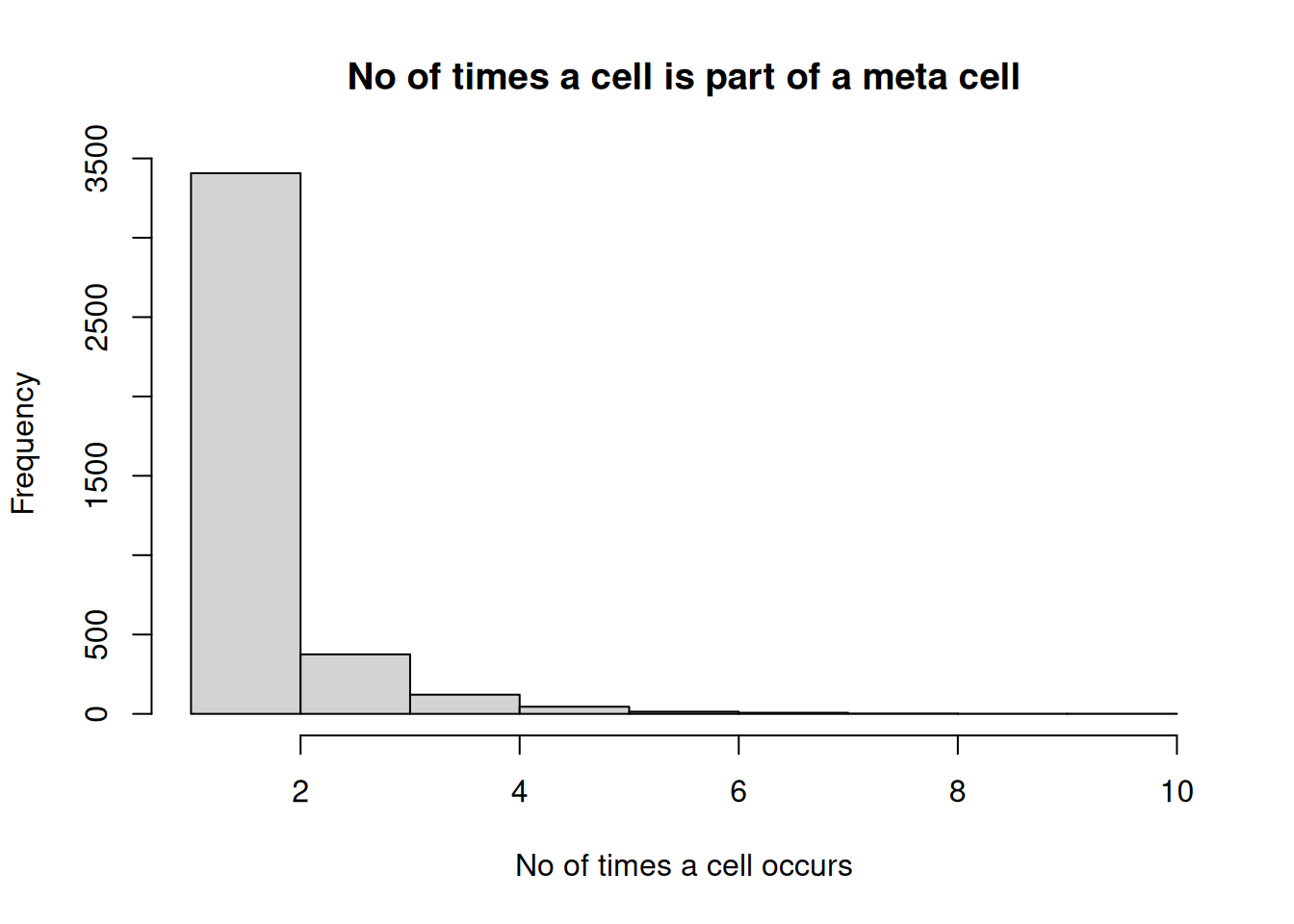
As we can appreciate, some of the cells are indeed shared across meta cells. Let’s add the diffusion coordinates to this one for later analysis
hdwgcna <- calc_diffusion_coordinates(object = hdwgcna, knn_data = knn_object)SEACells
SEACells operates on the PCA embedding (or any batch corrected embedding) and the kNN graph and runs an iterative kernel archetypal analysis. n_sea_cells sets the number of archetypes; min_iter/max_iter bound the optimisation; convergence_epsilon sets the early stopping threshold relative to the initial RSS. The algorithm was aggressively optimised to be faster. With pruning = TRUE (default) small values are set to zero, removing basically dust and accelerating the calculations substantially. The rule of thumb by the authors is one SEACell per 75 cells, i.e., 90 SEACells for this experiment. We will set this higher here to 250L to make this a bit more comparable with the other methods…
seacells <- generate_seacells_sc(
  object = sc_object,
  seacell_params = params_sc_seacells(
    n_sea_cells = 250L,
    min_iter = 10L,
    convergence_epsilon = 0.001
  ),
  .verbose = TRUE
)

seacells
#> Single cell experiment (Meta Cells).
#>   Meta cell method: seacell
#>   Merged: FALSE
#>   No meta cells: 250
#>   No genes: 12464
#>   No cells aggregated: 6881
#>   No obs rows in source: 6881
#>   HVG calculated: FALSE
#>   PCA calculated: FALSE
#>   Other embeddings: none
#>   KNN generated: FALSE
#>   SNN generated: FALSE
#>   Stale artefacts: none
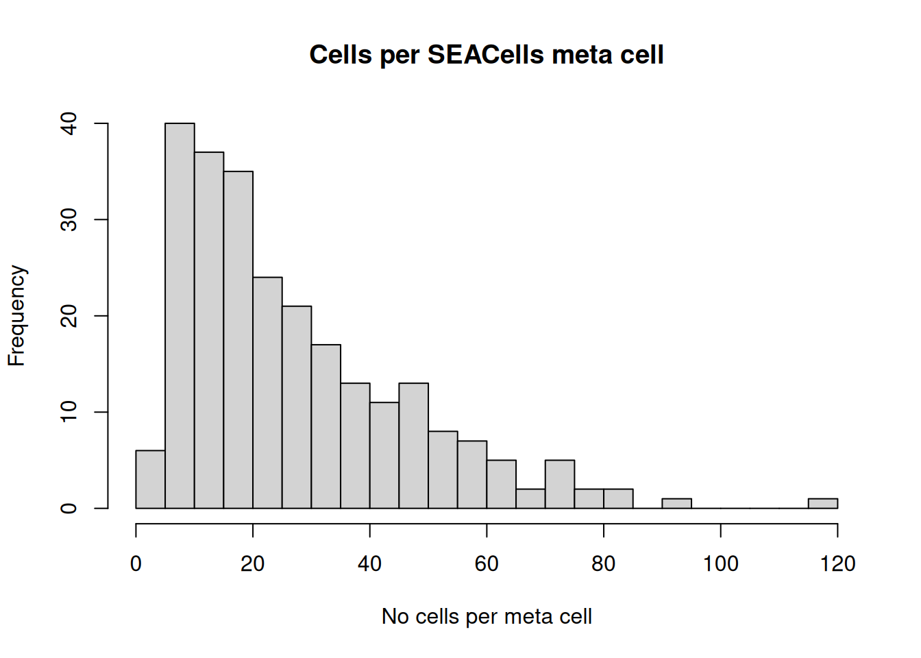
We can appreciate that each SEACell can contain a varying degree of original cells contributing to this specific metacell.
no_cells_seacells <- purrr::map_dbl(seacells[[]]$original_cell_idx, length)

hist(
  no_cells_seacells,
  xlab = "No cells per meta cell",
  main = "Cells per SEACells meta cell",
  breaks = 25L
)
We will also add the diffusion coordinates to this one
seacells <- calc_diffusion_coordinates(object = seacells, knn_data = knn_object)SEACells on large data
SEACells is infamous for being very slow and difficult to run on larger data sets. Most of the hot path has been rewritten in bixverse, which is what makes the algorithm feasible beyond a few tens of thousands of cells:
- The initialisation is the part of the original algorithm that scales the worst. The greedy column subset selection needs a full
K^2column for every candidate cell, which isO(N^2)and simply will not finish on millions of cells.bixversetherefore switches strategy by size: abovegreedy_threshold(20,000 cells by default) it drops the greedy top-up and samples the archetypes at random, which is effectively free. When a better-than-random start is wanted but the greedy pass is still out of reach, settingn_landmarksenables a Nyström route: a small set of density-weighted landmarks is chosen (5 to 10 timesn_sea_cellsis a sensible range), the diffusion operator is built and eigendecomposed on those landmarks alone, and the multiscale embedding is carried to all cells via a Nyström extension before the usual max-min waypoint sampling. The eigendecomposition stays at landmark scaleL x Linstead ofN x N. - The optimisation loop itself runs in bounded memory.
K^2is never formed; everyK^2 Xterm is evaluated asK (K X), so memory stays bounded by the number of non-zeros inKrather thanN^2. Neither Frank-Wolfe gradient is ever materialised. The A update runs cell-major: a column ofAis a convex combination of at mostmax_fw_itersone-hot atoms, so the solver carries(index, weight)pairs and patches the gradient with rank-1 corrections instead of rebuilding it from the sparseAon every iteration. The argmin over the two gradient terms is fused and runs on SIMD (NEON on Apple Silicon, SSE2, AVX-2 or AVX-512 picked at runtime on x86). The B update walks one gradient column per archetype in the same spirit. Everything is chunked across rayon threads. -
K^2 Bis the one product the inner loop needs on every single iteration, so it is cached rather than recomputed. A Frank-Wolfe step changesBby a rank-k update, and the matching change toK^2 Bis the same scaling plus one weighted column ofK^2per archetype; the pruning corrections fold into the same delta. The update is exact, and a full recompute still runs every eight iterations to bound floating point drift and the sparsity pattern. The B loop stops early once the relative Frank-Wolfe duality gap drops below1e-3. -
pruningis on by default and should stay on. The Frank-Wolfe updates only ever add atoms, so without pruning the non-zeros inAandBclimb monotonically across the whole fit and the time per iteration keeps rising instead of settling. The accuracy cost sits inpruning_threshold, not in the flag. Keep it below the smallest weight the schedule can produce,2 / (T (T + 1))forT = max_fw_iters; above that you start deleting live mass and shift the solution. The default1e-7removes numerical dust only. - The RSS for the convergence check never materialises the
N x NreconstructionK B A. The squared residual is expanded with the trace identity and evaluated through cyclic reordering, so every intermediate is at mostN x kork x k. Same Frobenius norm, just without the dense reconstruction.
Most of that is automatic. The knobs you actually reach for on large data are greedy_threshold and n_landmarks for the initialisation, and pruning/pruning_threshold for the loop. Together they are what made it possible to run a million cells locally, which the original implementation cannot do.
SuperCells
SuperCells runs walktrap on the kNN graph. The number of meta cells is set indirectly through graining_factor: with a factor of 30 over ~6800 cells you should get roughly ~230 meta cells. The option to run the kernel-based version of SuperCells 2.0 from Hérault et al. is enabled by default. (The multi-modal versions are still to come. Watch the space…)
supercells <- generate_supercells_sc(
  object = sc_object,
  sc_supercell_params = params_sc_supercell(
    graining_factor = 30
  ),
  .verbose = TRUE
)

supercells
#> Single cell experiment (Meta Cells).
#>   Meta cell method: supercells
#>   Merged: FALSE
#>   No meta cells: 230
#>   No genes: 12464
#>   No cells aggregated: 6881
#>   No obs rows in source: 6881
#>   HVG calculated: FALSE
#>   PCA calculated: FALSE
#>   Other embeddings: none
#>   KNN generated: FALSE
#>   SNN generated: FALSE
#>   Stale artefacts: none
Let’s plot the number of cells per SuperCell.
no_cells_supercells <- purrr::map_dbl(supercells[[]]$original_cell_idx, length)

hist(
  no_cells_supercells,
  xlab = "No cells per meta cell",
  main = "Cells per Supercell",
  breaks = 25L
)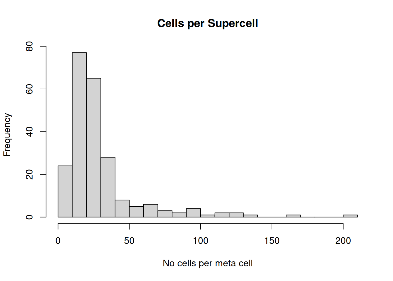
Similar to SEACells, we get a gradient here.
supercells <- calc_diffusion_coordinates(
  object = supercells,
  knn_data = knn_object
)
SuperCells on large data
SuperCell is already far cheaper than SEACells on large data: there is no archetypal analysis, just Walktrap community detection on the kNN graph. The one part that does not scale naively is the random-walk representation. compute_walk_probabilities() within the Rust code gives every cell a sparse vector of landing probabilities for a walk_length-step walk; on a well-connected graph these vectors spread to touch a large fraction of cells after only a few steps, so the store drifts towards dense and memory grows as O(n × support).
max_support caps this. With max_support = k each initial walk vector keeps only its k largest entries (the dropped tail holds negligible walk mass), bounding the store at roughly k × n regardless of how far the walks spread. This makes the run an approximation: the Ward merge criterion is driven by distances between walk vectors, and truncating them can shift the merge order slightly, so you may get marginally different communities than the exact run. With max_support = NULL (the default) the walks are kept exact. Beyond saving memory, a smaller k also speeds up every distance and merge operation, since both are linear in the support.
supercells_large <- generate_supercells_sc(
  object = sc_object,
  sc_supercell_params = params_sc_supercell(
    graining_factor = 30,
    max_support = 256L # would bound the walk vectors to 256
  ),
  .verbose = TRUE
)
Metrics
Purity
A simple sanity check is to ask, for each meta cell, what fraction of its constituent cells share the same underlying label. We use the Leiden clusters from the parent SingleCells object as a proxy for cell type identity. The labels themselves are imperfect, so absolute numbers should be read with that caveat, but relative differences between methods are reasonably indicative.
# memberships are positions in the full obs table, so the labels have to come
# from the unfiltered obs rather than from `sc_object[[...]]`
cell_labels <- as.character(get_sc_obs(sc_object)$celltype)

hdwgcna <- calc_meta_cell_purity(hdwgcna, original_cell_type = cell_labels)
seacells <- calc_meta_cell_purity(seacells, original_cell_type = cell_labels)
supercells <- calc_meta_cell_purity(
  supercells,
  original_cell_type = cell_labels
)

purity_dt <- rbind(
  data.table(method = "hdWGCNA", purity = hdwgcna[[]]$mc_purity),
  data.table(method = "SEACells", purity = seacells[[]]$mc_purity),
  data.table(method = "SuperCells", purity = supercells[[]]$mc_purity)
)

purity_dt[, .(mean = mean(purity), median = median(purity)), by = method]
#>        method      mean    median
#>        <char>     <num>     <num>
#> 1:    hdWGCNA 0.8838462 0.9615385
#> 2:   SEACells 0.9026757 1.0000000
#> 3: SuperCells 0.8944299 0.9784323
ggplot(purity_dt, aes(x = method, y = purity)) +
  geom_violin(aes(fill = method), alpha = 0.6) +
  geom_boxplot(width = 0.05, outlier.size = 0.5) +
  theme_bw() +
  theme(legend.position = "none") +
  labs(x = "Method", y = "Meta cell purity (Leiden)") +
  ylim(0, 1)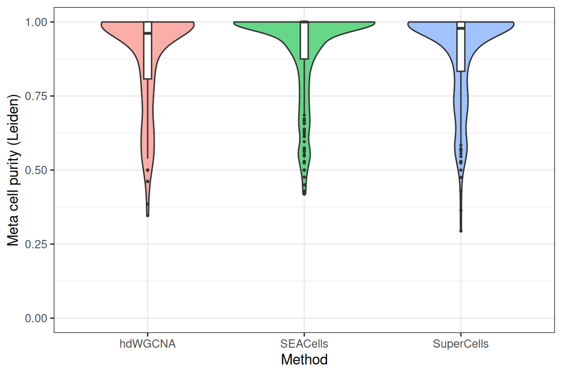
In terms of cell type purity, the methods are basically the same. Potentially more interesting is their behaviour in the manifold, see below…
Manifold regions
We called the calc_diffusion_coordinates() with the kNN graph on the data. This will tell us which parts of the manifold are being sampled here, i.e., for example high, medium or low density regions (based on the diffusion map and distance to the 150k-th neighbour within that). This gives an idea how many rare cell states the meta cells capture.
hdwgcna_regions <- as.data.table(
  table(hdwgcna[[]]$density_region) / nrow(hdwgcna[[]])
)[, method := "hdWGCNA"]
seacells_regions <- as.data.table(
  table(seacells[[]]$density_region) / nrow(seacells[[]])
)[, method := "SEACells"]
supercells_regions <- as.data.table(
  table(supercells[[]]$density_region) / nrow(supercells[[]])
)[, method := "SuperCells"]

region_dt <- rbind(
  hdwgcna_regions,
  seacells_regions,
  supercells_regions
)[, V1 := factor(V1, levels = c("high", "mid", "low"))]
setnames(region_dt, old = c("V1", "N"), new = c("region", "proportion"))
ggplot(region_dt, aes(x = method, y = proportion, fill = region)) +
  geom_bar(stat = "identity") +
  theme_bw() +
  labs(x = "Method", y = "Proportion of meta cells", fill = "Density region") +
  scale_fill_manual(
    values = setNames(
      c("#2c2d54", "#969bc7", "#6f9954"),
      c("high", "mid", "low")
    )
  )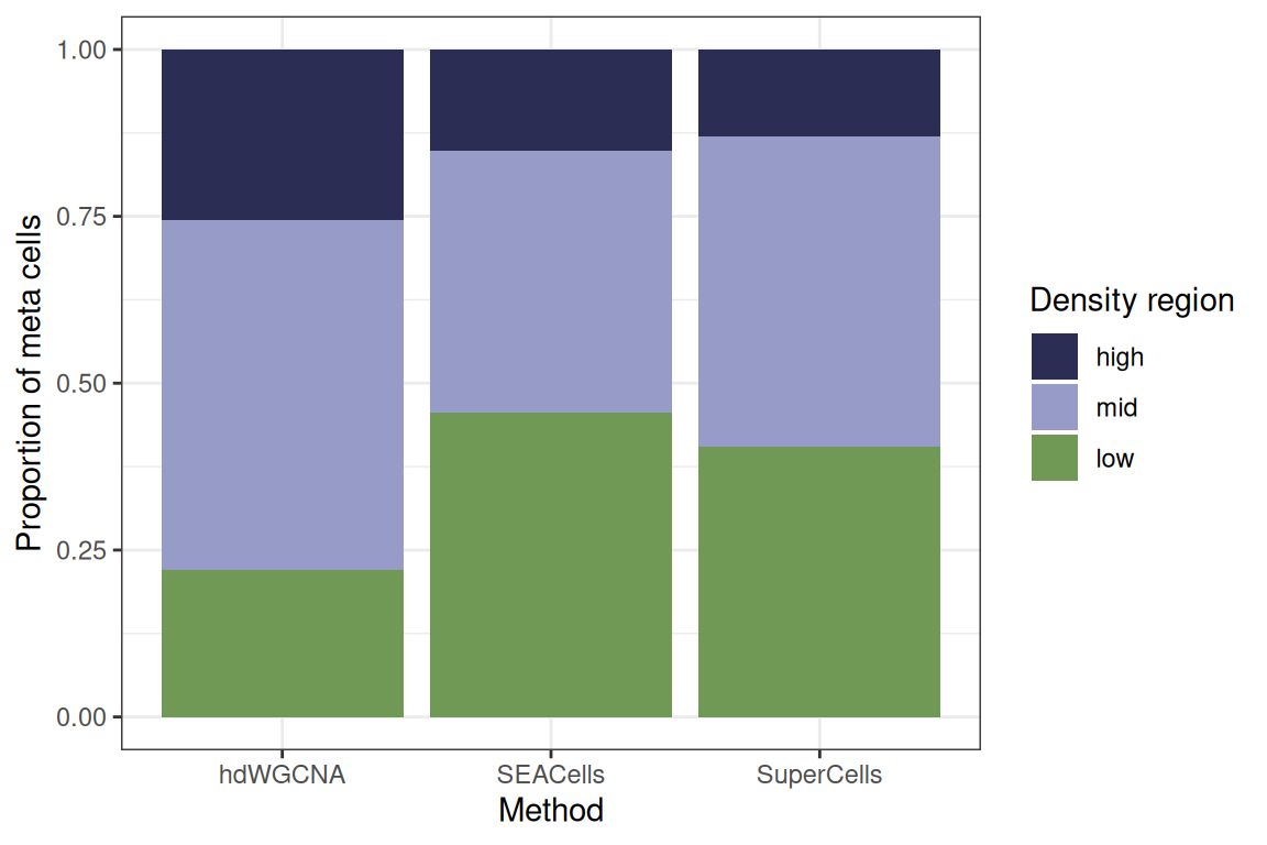
This is one of the most important differences between the methods. hdWGCNA will disproportionally sample regions of the manifolds with medium density and basically proportion-based. SEACells on the other hand generates meta cells that capture sparse (more heterogenous) regions of the manifold. SuperCells sits between the two methods.
Compactness and separation
We can also assess other metrics on the manifold representation. Compactness (how close are the cells within a given metacell to the centroid) and separation (how far is the closest centroid). The first gives an (unbiased) indication of purity; the latter of diversity captured in the manifold. We can do this trivially via:
hdwgcna <- calc_manifold_metrics(hdwgcna)
seacells <- calc_manifold_metrics(seacells)
supercells <- calc_manifold_metrics(supercells)
Let’s generate a plotting data.table
metrics_dt <- rbind(
  data.table(
    method = "hdWGCNA",
    separation = hdwgcna[[]]$separation,
    compactness = hdwgcna[[]]$compactness,
    region = hdwgcna[[]]$density_region
  ),
  data.table(
    method = "SEACells",
    separation = seacells[[]]$separation,
    compactness = seacells[[]]$compactness,
    region = seacells[[]]$density_region
  ),
  data.table(
    method = "SuperCells",
    separation = supercells[[]]$separation,
    compactness = supercells[[]]$compactness,
    region = supercells[[]]$density_region
  )
)[, region := factor(region, levels = c("high", "mid", "low"))]

metrics_dt[,
  .(
    mean_separation = mean(separation),
    median_separation = median(separation),
    mean_compactness = mean(compactness),
    median_compactness = median(compactness)
  ),
  .(method)
]
#>        method mean_separation median_separation mean_compactness
#>        <char>           <num>             <num>            <num>
#> 1:    hdWGCNA       0.2296308         0.1619662       0.04015360
#> 2:   SEACells       0.2951381         0.2243744       0.04030184
#> 3: SuperCells       0.3235611         0.2823487       0.03296062
#>    median_compactness
#>                 <num>
#> 1:         0.02346519
#> 2:         0.02231498
#> 3:         0.01786626
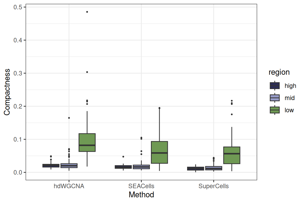
Some differences are visible here. hdWGCNA has the worst separation and best compactness (not unexpected given the bootstrapping method only sampling direct neighbours). SEACells has the worst compactness across the three methods (not unsurprising as the meta cells here capture more sparse regions of the manifold) and middling separation; SuperCells (version 2.0, the default setting here) is in the middle.
per_region_stats <- metrics_dt[,
  .(
    mean_separation = mean(separation),
    median_separation = median(separation),
    mean_compactness = mean(compactness),
    median_compactness = median(compactness)
  ),
  .(method, region)
]
setorder(per_region_stats, method, region)

per_region_stats[]
#>        method region mean_separation median_separation mean_compactness
#>        <char> <fctr>           <num>             <num>            <num>
#> 1:   SEACells   high      0.07419151        0.07158697       0.01718058
#> 2:   SEACells    mid      0.24898195        0.19595428       0.01953950
#> 3:   SEACells    low      0.40846499        0.36357117       0.06585726
#> 4: SuperCells   high      0.08978874        0.09189881       0.01214339
#> 5: SuperCells    mid      0.26108687        0.24177319       0.01418879
#> 6: SuperCells    low      0.47085039        0.45609254       0.06127356
#> 7:    hdWGCNA   high      0.06160547        0.05265780       0.02189890
#> 8:    hdWGCNA    mid      0.19093212        0.17392720       0.02312327
#> 9:    hdWGCNA    low      0.51732464        0.43812355       0.10195858
#>    median_compactness
#>                 <num>
#> 1:         0.01563445
#> 2:         0.01640135
#> 3:         0.05865810
#> 4:         0.01180709
#> 5:         0.01166381
#> 6:         0.05646008
#> 7:         0.02150713
#> 8:         0.01998665
#> 9:         0.08192069
We can also look at this per density region in the manifold where we can observe that compactness is smallest in the high density regions, whereas separation is the highest in the low density regions. And below as plots:
Compactness plots
ggplot(metrics_dt, aes(x = method, y = compactness)) +
  geom_violin(aes(fill = method), alpha = 0.6) +
  geom_boxplot(width = 0.05, outlier.size = 0.5) +
  theme_bw() +
  theme(legend.position = "none") +
  labs(x = "Method", y = "Compactness")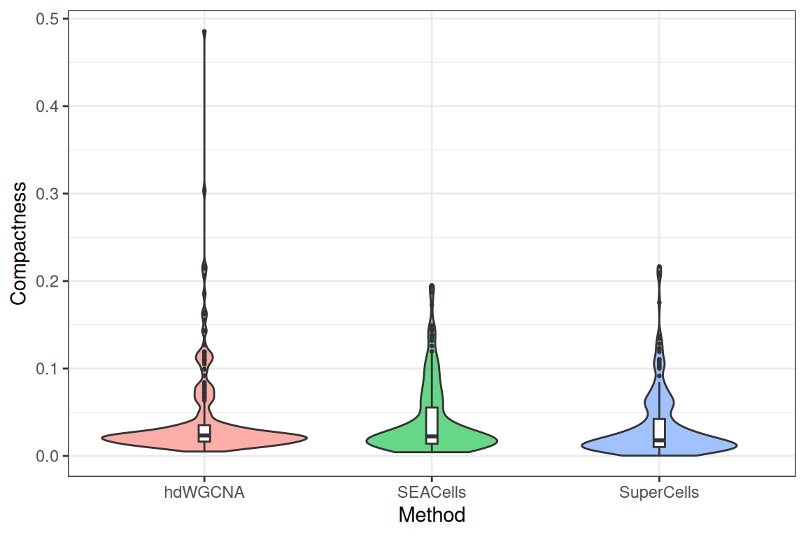
ggplot(metrics_dt, aes(x = method, y = compactness)) +
  geom_boxplot(aes(fill = region), outlier.size = 0.5) +
  theme_bw() +
  labs(x = "Method", y = "Compactness") +
  scale_fill_manual(
    values = setNames(
      c("#2c2d54", "#969bc7", "#6f9954"),
      c("high", "mid", "low")
    )
  )
Separation plots
ggplot(metrics_dt, aes(x = method, y = separation)) +
  geom_violin(aes(fill = method), alpha = 0.6) +
  geom_boxplot(width = 0.05, outlier.size = 0.5) +
  theme_bw() +
  theme(legend.position = "none") +
  labs(x = "Method", y = "Separation")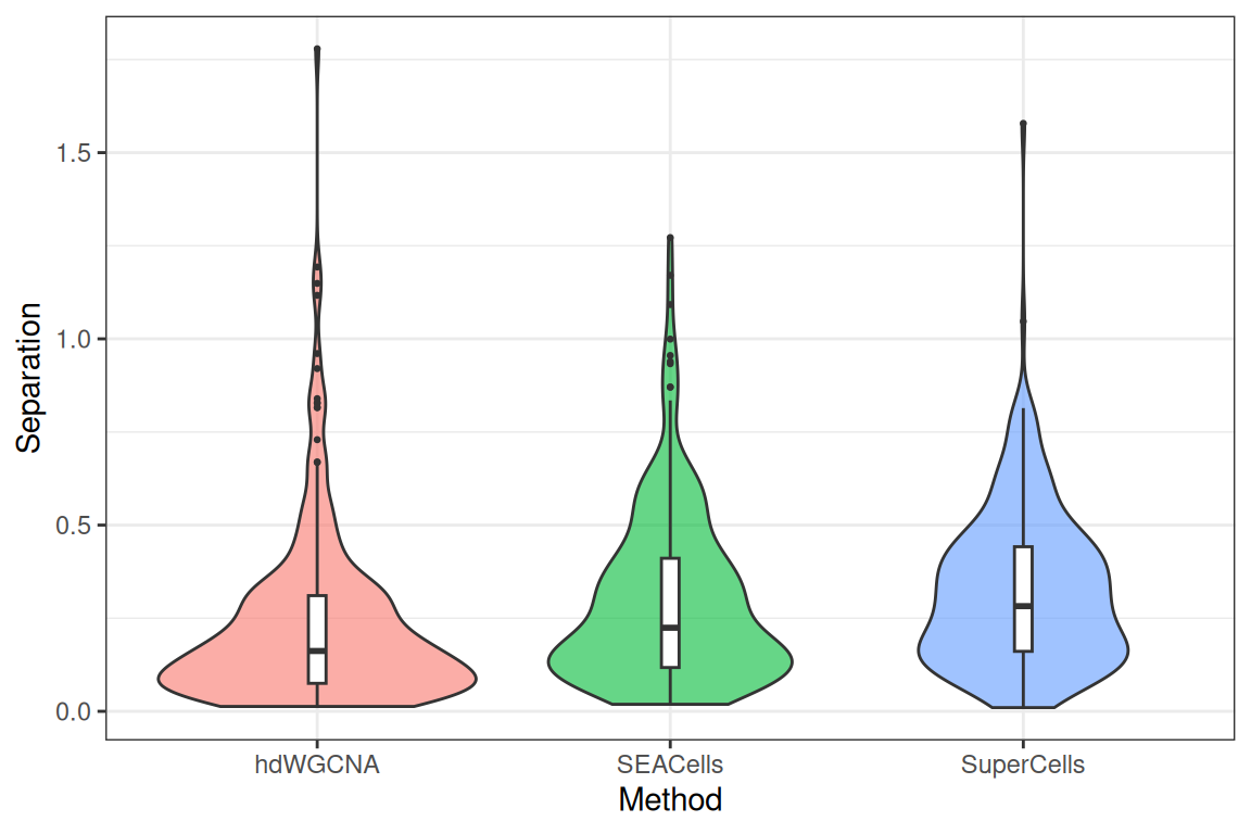
ggplot(metrics_dt, aes(x = method, y = separation)) +
  geom_boxplot(aes(fill = region), outlier.size = 0.5) +
  theme_bw() +
  labs(x = "Method", y = "Compactness") +
  scale_fill_manual(
    values = setNames(
      c("#2c2d54", "#969bc7", "#6f9954"),
      c("high", "mid", "low")
    )
  )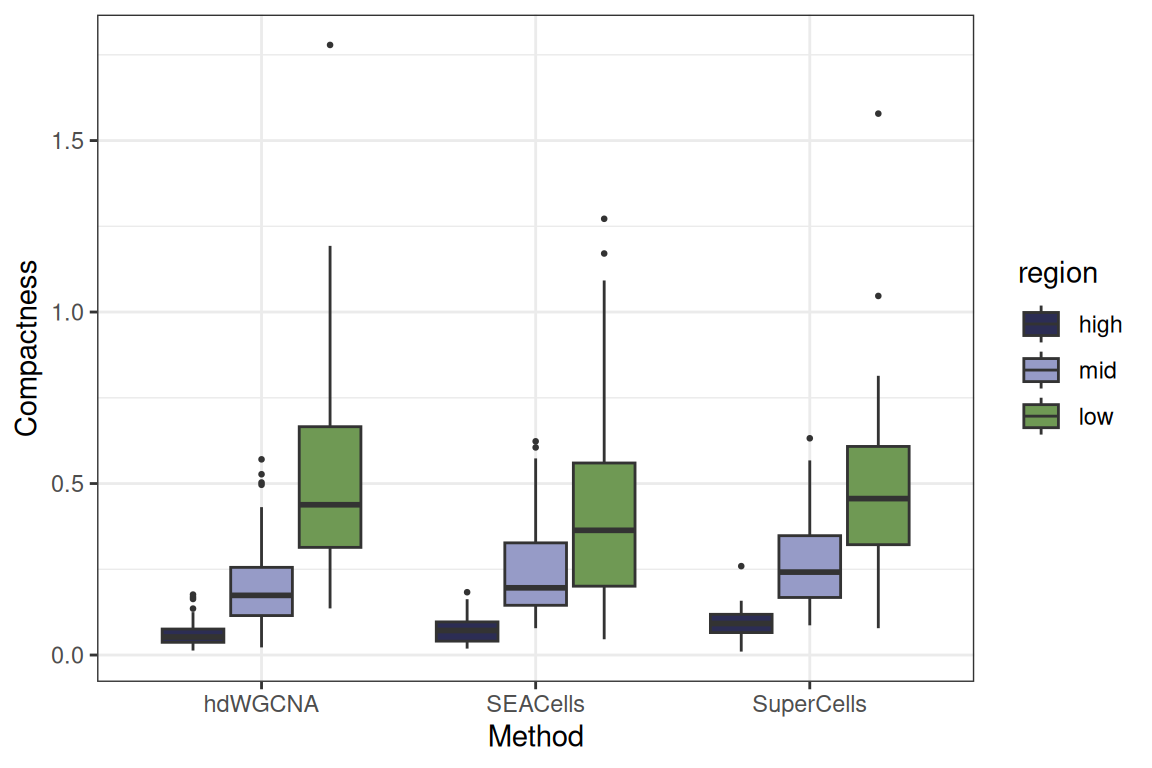
Based on this, we can conclude the following:
- Purity is VERY similar across the methods (for this data set).
- At matched K (~250 metacells), SuperCells achieves the lowest median compactness, slightly ahead of hdWGCNA and SEACells. Separation is comparable between SuperCells and SEACells, with hdWGCNA noticeably lower.
- The methods differ markedly in where they place metacells. SEACells assigns 50% of metacells to low-density regions versus 24% for hdWGCNA and 41% for SuperCells, consistent with its kernel archetypal formulation seeking out underrepresented states.
- Method choice should reflect the downstream question. For tight aggregation in dense regions (e.g., bulk-like pseudo-replicates of common cell types), SuperCells is efficient and effective. For preserving rare populations or transitioning states (e.g., differentiation trajectories), SEACells’ rare-state bias is desirable, with the trade-off of more heterogeneous metacells in those regions. hdWGCNA is fast and simple but assignments overlap more in embedding space.
Working with the MetaCells class
This is where the in-memory representation pays off. HVG selection, PCA, neighbour graphs and embeddings on a few hundred meta cells take seconds and do not touch the Rust binary files on disk. We will just take forward SEACells here, but the methods below work across all of MetaCells.
HVGs and PCA
The same HVG and PCA method dispatches you know from single cells work here…
seacells <- find_hvg_sc(
  object = seacells,
  hvg_no = 2000L,
  .verbose = FALSE
)

seacells <- calculate_pca_sc(
  object = seacells,
  no_pcs = 30L
)
Neighbours, clustering and UMAP
And also the same interfaces for neighbours, (Leiden) clustering and UMAP can be used here.
seacells <- find_neighbours_sc(
  object = seacells,
  neighbours_params = params_sc_neighbours(
    knn = list(k = 10L, knn_method = "exhaustive")
  )
)
#>
#> Generating sNN graph (full: TRUE).
#> Transforming sNN data to igraph.

seacells <- find_clusters_sc(seacells, res = 1.0, name = "leiden_clusters")

seacells <- umap_sc(seacells, k = 10L, knn_method = "exhaustive")
#> Running UMAP.
#> Using n_epochs = 500 (dataset <10k samples or adam_parallel optimiser)
#> Using provided kNN graph.
embedding_plot_sc(
  object = seacells,
  embedding = "umap",
  colour_by = "leiden_clusters",
  discrete = TRUE
)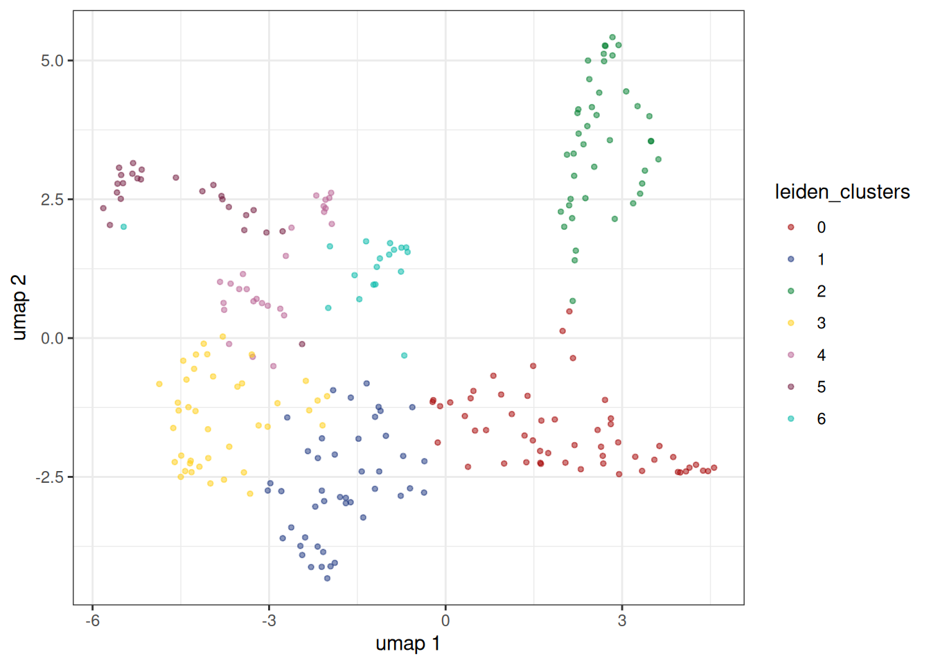
The plot is much sparser than the equivalent UMAP on the original cells, which is the point: each dot is a denoised aggregate of ~15-20 cells, and the structure that survives aggregation is the structure that’s robust to sparsity.
Co-expression module detection on meta cells
Meta cells compress information and reduce sparsity. That makes them ideal for co-expression module detection methods and we can use a SCENIC implementation within bixverse akin to the single cell version also on MetaCells.
Let’s run this quickly…
tf_dt <- data.table::fread(
  "https://resources.aertslab.org/cistarget/tf_lists/allTFs_hg38.txt",
  header = FALSE,
  col.names = "tf"
)

scenic_res <- scenic_grn_sc(
  object = seacells,
  tf_ids = tf_dt$tf,
  scenic_params = params_scenic(
    learner_type = "randomforest",
    gene_batch_size = 64L,
    # due to the small data set size, we should set 'min_samples_leaf' lower
    # than for a massive single cell data set
    learner_params = list(min_samples_leaf = 10L)
  ),
  .verbose = TRUE
)
#> No target genes supplied, running gene filter...
#> SCENIC gene filter: 12464 / 12464 genes pass.
#> Warning in `method(scenic_grn_sc, bixverse::MetaCells)`(object = <object>, :
#> 610 TF identifier(s) not found in the object and dropped.
#> SCENIC: 12464 target genes, 1282 TFs, 250 cells
scenic_res <- identify_tf_to_genes(
  scenic_res,
  n_sd = 2,
  .verbose = TRUE
)
#> Extracting TF to gene associations via per-gene threshold (mean + 2.0 * SD).

scenic_res <- tf_to_genes_correlations(
  x = scenic_res,
  object = seacells,
  .verbose = TRUE
)
#> Calculating the pairwise correlations between the TFs and genes
#> Keeping activating TF <> gene links at |rho| > 0.030
#> Removing self loops (TF controlling its own expression

# no motif filter here, so the leading edge column does not exist yet
tf_to_gene_ls <- build_regulons(scenic_res, use_leading_edge = FALSE)
#> Built 587 regulons (124 dropped below 10 genes). Median size: 311
In a proper situation we would filter down the TF to gene associations via motifs, please refer to the details in this vignette. We will skip this step for now and just run AUCell to show how it works. Which statistic you get is controlled by params_sc_aucell(). The default is "recovery", the original AUCell recovery curve, which is what SCENIC uses. "wilcox" (Mann-Whitney AUC over the full ranking) and "ap" (average precision) are the other two options.
auc_res <- aucell_sc(
  object = seacells,
  gs_list = tf_to_gene_ls,
  aucell_params = params_sc_aucell()
)

umap_dt <- as.data.table(
  get_embedding(seacells, "umap"),
  keep.rownames = "meta_cell_id"
)

umap_dt[, `:=`(IRF1 = auc_res[, "IRF1"], TCF4 = auc_res[, "TCF4"])]

p1 <- ggplot(umap_dt, aes(x = umap_1, y = umap_2)) +
  geom_point(aes(fill = IRF1), size = 2.5, shape = 21) +
  theme_bw() +
  labs(fill = "IRF1 AUC") +
  scale_fill_viridis_c()

p2 <- ggplot(umap_dt, aes(x = umap_1, y = umap_2)) +
  geom_point(aes(fill = TCF4), size = 2.5, shape = 21) +
  theme_bw() +
  labs(fill = "TCF4 AUC") +
  scale_fill_viridis_c()

p1 + p2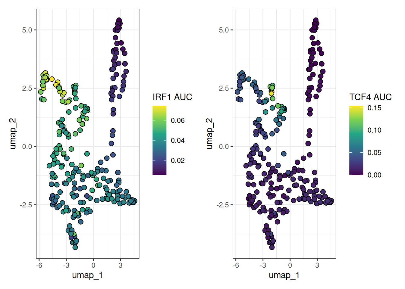
Consensus NMF on meta cells
The same argument applies to matrix factorisation, and here compression buys you something concrete. Consensus NMF (Kotliar, et al.) fits n_runs NMFs, pools their components, drops the ones sitting on their own, clusters the survivors and takes the median of each cluster. What survives is the programme structure the restarts agree on. The catch on raw single cells is memory: every restart is dense, and they all live at once. On a few thousand meta cells rather than a few hundred thousand cells, n_runs = 50 is unremarkable. This is the path where consensus NMF is genuinely affordable.
Start by picking k. nmf_k_sweep_sc() runs the consensus step across a range of ranks and reports stability against reconstruction error, keeping no factors.
mc_k_sweep <- nmf_k_sweep_sc(
  object = seacells,
  k_range = 2:12,
  n_runs = 10L,
  nmf_consensus_params = params_nmf_consensus(density_threshold = 2)
)

mc_k_sweep
#> NmfKSweepResult (consensus NMF k sweep)
#>   Source class:     MetaCells
#>   k range:          2 to 12
#>   No runs per k:    10
#>   Most stable k:    3 (stability = 0.9995)
#>
#>         k stability best_error median_error consensus_failed n_dropped
#>     <int>     <num>      <num>        <num>           <lgcl>     <int>
#>  1:     2 0.9966910 0.16070975   0.16071980            FALSE         0
#>  2:     3 0.9994817 0.12868318   0.12868918            FALSE         0
#>  3:     4 0.9977547 0.11222275   0.11224078            FALSE         0
#>  4:     5 0.9980604 0.10001751   0.10004166            FALSE         0
#>  5:     6 0.9984983 0.09023863   0.09026857            FALSE         0
#>  6:     7 0.8303745 0.08418021   0.08623367            FALSE         0
#>  7:     8 0.8122041 0.08008617   0.08037786            FALSE         0
#>  8:     9 0.8405823 0.07643273   0.07652184            FALSE         0
#>  9:    10 0.8395775 0.07274825   0.07285794            FALSE         0
#> 10:    11 0.8326951 0.07063823   0.07079682            FALSE         0
#> 11:    12 0.7905937 0.06896664   0.06926464            FALSE         0
#>     n_empty_clusters n_converged
#>                <int>       <int>
#>  1:                0          10
#>  2:                0          10
#>  3:                0          10
#>  4:                0          10
#>  5:                0          10
#>  6:                0          10
#>  7:                0          10
#>  8:                0          10
#>  9:                0          10
#> 10:                0          10
#> 11:                0          10
plot(mc_k_sweep)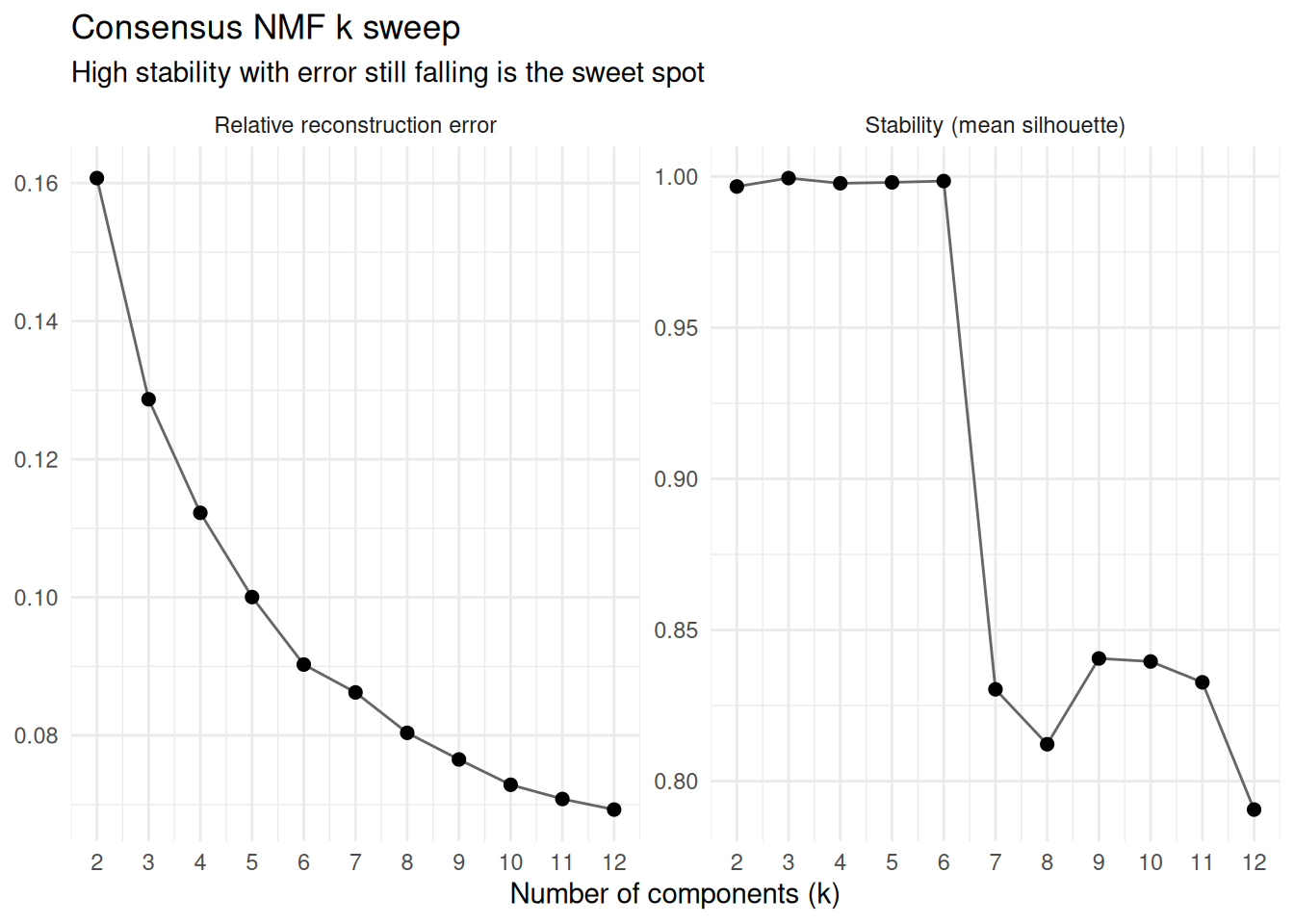
The usual rule is to take the last k before stability falls away, while the error curve is still coming down. Here it does not fall away so much as bounce: stability stays high across the whole range and dips and recovers, which says the meta cells support several plausible ranks rather than one obvious answer. It peaks at 6 and the error is still coming down there, so that is where we fit.
mc_nmf <- consensus_nmf_sc(
  object = seacells,
  k = 6L,
  n_runs = 10L,
  nmf_consensus_params = params_nmf_consensus(density_threshold = 2)
)

mc_nmf
#> ConsensusNmfResult (consensus HALS NMF)
#>   Source class:     MetaCells
#>   No genes:         2000
#>   No cells:         250
#>   No components:    6
#>   No runs:          10
#>   Stability:        0.9437
#>   Relative error:   0.09026
#>   Dropped:          0 / 60 components
#>   Preprocessing:    none
get_stability() gives you the diagnostics: the mean silhouette of the clusters, the relative reconstruction errors, and a row per pooled component recording where it landed.
mc_nmf_diag <- get_stability(mc_nmf)
mc_nmf_diag$stability
#> [1] 0.9436891
mc_nmf_diag$cluster_sizes
#>    cluster     n
#>      <int> <int>
#> 1:       1    11
#> 2:       2    10
#> 3:       3     9
#> 4:       4    10
#> 5:       5    10
#> 6:       6    10
With 20 restarts, a cluster of 20 is a programme every run found. A thin one is a programme only some initialisations saw.
W (genes x k) and H (k x meta cells) come back in the same shape the single-run nmf_sc() gives you, so the activations drop straight onto the UMAP:
mc_h <- get_h(mc_nmf)

umap_nmf_dt <- as.data.table(
  get_embedding(seacells, "umap"),
  keep.rownames = "meta_cell_id"
)
umap_nmf_dt[, `:=`(
  comp_01 = mc_h["comp_01", meta_cell_id],
  comp_02 = mc_h["comp_02", meta_cell_id]
)]

p3 <- ggplot(umap_nmf_dt, aes(x = umap_1, y = umap_2)) +
  geom_point(aes(fill = comp_01), size = 2.5, shape = 21) +
  theme_bw() +
  labs(fill = "comp_01") +
  scale_fill_viridis_c()

p4 <- ggplot(umap_nmf_dt, aes(x = umap_1, y = umap_2)) +
  geom_point(aes(fill = comp_02), size = 2.5, shape = 21) +
  theme_bw() +
  labs(fill = "comp_02") +
  scale_fill_viridis_c()

p3 + p4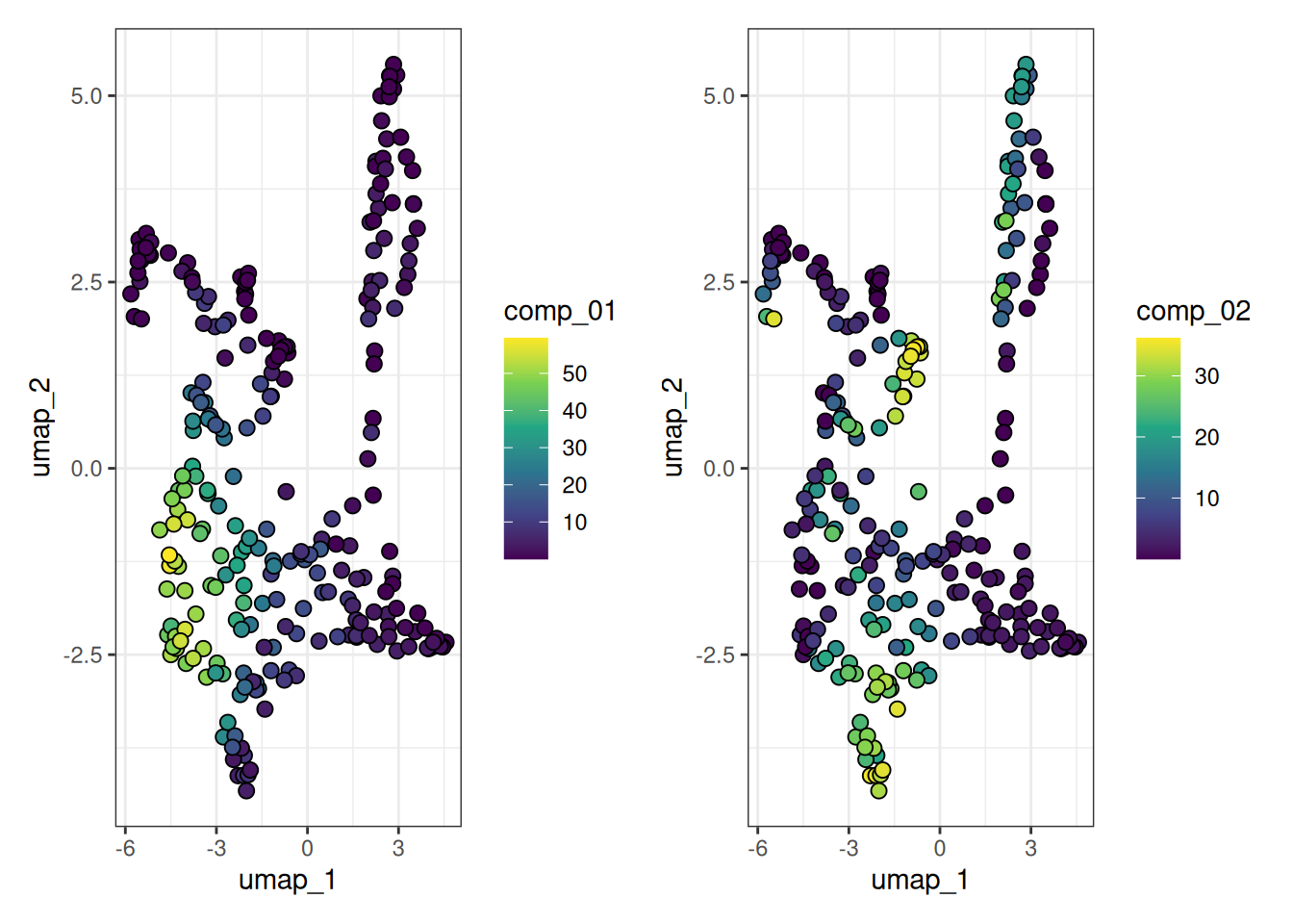
To read off what a programme is, rank the genes by their loading in W:
mc_w <- get_w(mc_nmf)

top_genes <- lapply(colnames(mc_w), \(comp) {
  names(sort(mc_w[, comp], decreasing = TRUE))[1:10]
})
names(top_genes) <- colnames(mc_w)
top_genes[1:3]
#> $comp_01
#>  [1] "MPO"    "ATP8B4" "AZU1"   "LRMDA"  "FNDC3B" "KCNQ5"  "ELANE"  "EREG"
#>  [9] "LYST"   "CSF3R"
#>
#> $comp_02
#>  [1] "DIAPH3" "ASPM"   "TOP2A"  "POLQ"   "RRM2"   "CIT"    "MKI67"  "NUSAP1"
#>  [9] "KIF15"  "AURKB"
#>
#> $comp_03
#>  [1] "IGLL1"      "MSI2"       "NEGR1"      "DNTT"       "MIR181A1HG"
#>  [6] "GAPDH"      "EBF1"       "PLCB1"      "RACK1"      "RPL12"
Pseudo-bulking
Pseudo-bulks are conceptually adjacent but solve a different problem. Where meta cells are dense aggregates designed to feed into co-expression and archetype methods, pseudo-bulks are coarse summaries (typically one bulk per sample-by-cluster combination) used as input to bulk-style DGE tools such as limma-voom, edgeR or DESeq2 to get around pseudo-replication problems and p-value inflation in cell-based DGEs, see Zimmerman et al.
get_pseudobulked_sc takes a named list of cell IDs and returns either a dense matrix or a sparse dgRMatrix. With assay = "raw" it sums raw counts (what bulk DGE tools expect); with assay = "norm" it averages normalised counts.
cl_dt <- sc_object[[c("leiden", "cell_id")]]
cell_list <- split(cl_dt$cell_id, cl_dt$leiden)

pb_counts <- get_pseudobulked_sc(
  object = sc_object,
  cell_list = cell_list,
  return_format = "sparse",
  assay = "raw",
  .verbose = FALSE
)

dim(pb_counts)
#> [1]    14 12464
The returned matrix has one row per group and one column per gene. From here the standard bulk DGE pipeline applies: transpose it and hand it to run_edger_ql() or run_limma_voom(), both in Rust, no edgeR or limma needed.
Clean up
unlink(tempdir_cd34, recursive = TRUE, force = TRUE)