
Trajectory inference with Palantir and PAGA
2026-09-24
Intro
Two trajectory methods live in bixverse, both operating on the kNN graph you already built with find_neighbours_sc().
Palantir (Setty et al., 2019) models differentiation as a Markov chain over a multiscale diffusion map of the cells. Out come a pseudotime per cell, the probability of each cell reaching each terminal state, and the differentiation entropy derived from those probabilities. It needs a start cell and, optionally, the terminal states.
PAGA (Wolf et al., 2019) abstracts the cell-level graph into a cluster-level one, where the edge weight between two clusters measures how much more connected they are than a random null model expects. Its maximum spanning forest is the backbone people usually draw. PAGA needs a clustering and nothing else.
The data set is the one from the Palantir sample notebook: 4142 human CD34+ bone marrow cells across 16106 genes, already filtered. Three lineages come out of it, erythroid, monocyte and dendritic cell, all seeded from a haematopoietic stem cell pool.
The two supporting pieces from that notebook are here too. MAGIC (van Dijk et al., 2018) smooths counts over the same kNN graph, which is what makes the marker plots readable. Gene trends fit a landmark Gaussian process per branch, the Mellon-based estimator the reference uses rather than the legacy GAM. Both are restricted to a gene subset in bixverse, for reasons spelled out where they come up.
Loading the data
marrow_path <- download_marrow_cd34()

read_h5ad_metadata(marrow_path)$dims
#>   obs   var
#>  4142 16106
The var index of this file is the gene symbol, so no Ensembl mapping is needed. Cell barcodes look like Run4_120703408880541, which matters later: the start cell and the terminal states from the reference notebook are given as barcodes.
sc_object <- SingleCells(dir_data = tempdir())

sc_object <- load_h5ad(
  object = sc_object,
  h5_path = marrow_path,
  sc_qc_param = params_sc_min_quality(
    min_unique_genes = 100L,
    min_lib_size = 250L,
    min_cells = 10L,
    target_size = 10000
  )
)
#>  Using light streaming for the CSR to CSC conversion.
#> Loading observations data from h5ad into the DuckDB.
#> Loading variables data from h5ad into the DuckDB.

sc_object
#> Single cell experiment (Single Cells).
#>   No cells (original): 4142
#>    To keep n: 4142
#>   No genes: 14502
#>   HVG calculated: FALSE
#>   PCA calculated: FALSE
#>   Other embeddings: none
#>   KNN generated: FALSE
#>   SNN generated: FALSE
#>   MAGIC imputed: none
#>   Residual model: none
#>   Stale artefacts: none
The data ships pre-filtered, so there is no QC step here. On your own data you would run run_cell_qc() and set_cells_to_keep() first, as in the PBMC vignette.
Feature selection, PCA and neighbours
Standard pipeline. The one choice worth spelling out is k = 30 on the kNN graph: Palantir builds its diffusion kernel from whatever graph is stored on the object, and 30 neighbours is what the reference uses. The distance metric has to be euclidean, since the diffusion kernel is a Gaussian over a metric distance and cosine is not one.
pruning has to move with k. The default of 1/12 is set for the default k = 15, and since the threshold is a share of the neighbourhood, leaving it alone at k = 30 prunes twice as hard. Nothing errors, you just get cells with too few shared neighbours dropping out as one-cell clusters.
sc_object <- find_hvg_sc(
  object = sc_object,
  hvg_no = 1500L
)

sc_object <- calculate_pca_sc(
  object = sc_object,
  no_pcs = 30L
)
#> Using dense SVD solving on scaled data on 1500 HVG.

sc_object <- find_neighbours_sc(
  object = sc_object,
  neighbours_params = params_sc_neighbours(
    pruning = 1 / 24,
    knn = list(k = 30L, ann_dist = "euclidean")
  )
)
#>
#> Generating sNN graph (full: TRUE).
#> Transforming sNN data to igraph.

sc_object <- find_clusters_sc(
  sc_object,
  res = 0.7,
  name = "leiden_clusters"
)

sc_object <- umap_sc(sc_object)
#> Running UMAP.
#> Using n_epochs = 500 (dataset <10k samples or adam_parallel optimiser)
#> Using provided kNN graph.
embedding_plot_sc(
  sc_object,
  embedding = "umap",
  colour_by = "leiden_clusters",
  label_by = "leiden_clusters",
  discrete = TRUE
)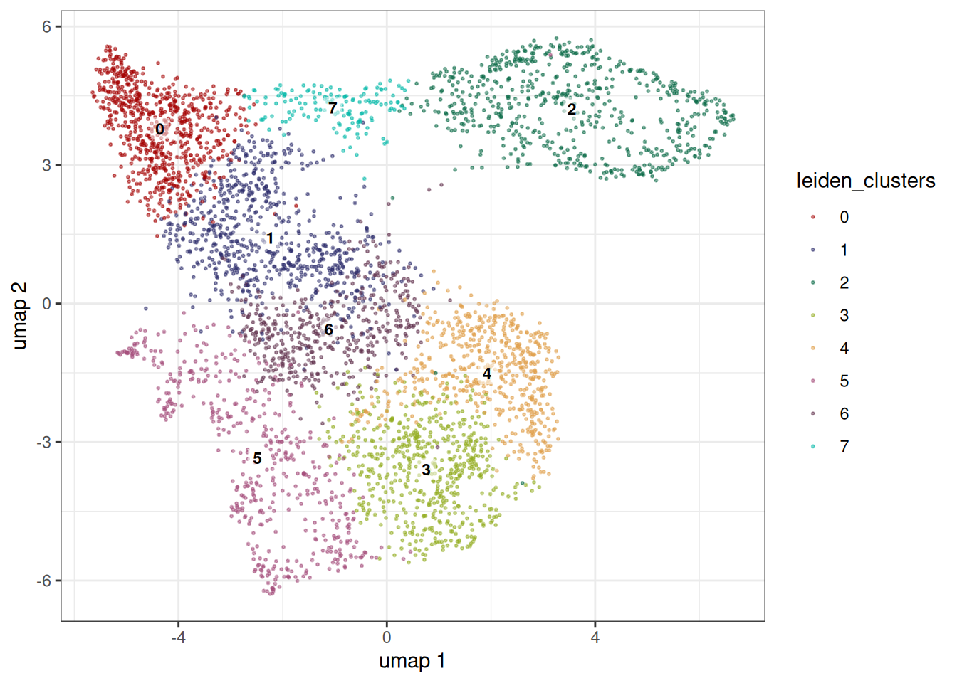
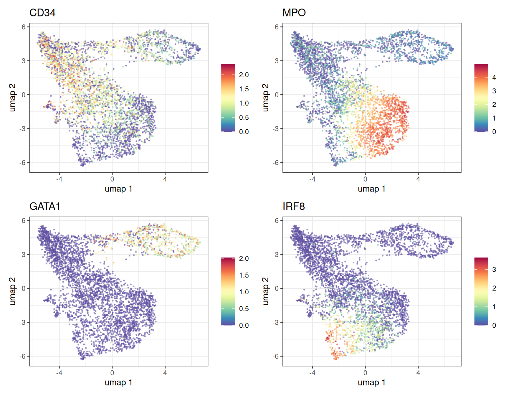
The four markers the reference notebook uses: CD34 for the stem pool, MPO for the myeloid arm, GATA1 for the erythroid one and IRF8 for the dendritic one. Raw, these are sparse and speckled, but the gradients are visible.
markers <- c("CD34", "MPO", "GATA1", "IRF8")

feature_plot_sc(
  object = sc_object,
  features = markers,
  embedding = "umap",
  palette = "spectral"
)
MAGIC imputation
MAGIC builds a row-stochastic operator over the kNN graph and applies it three times, so every cell becomes a weighted average of its neighbourhood. It is the same adaptive-bandwidth kernel Palantir uses for its diffusion map, so the two agree on what a neighbourhood is.
run_magic_sc() writes the result onto the object as a cached layer. It takes a gene list rather than doing everything, and that is deliberate: the output is dense, and the whole point of the on-disk store is not holding a dense cells-by-genes matrix. Pick the genes you want to look at.
sc_object <- run_magic_sc(sc_object, features = markers)
#> Running MAGIC over the rna kNN graph (4142 cells, 4 genes, 3 steps).

get_magic(sc_object)
#> ScMagic: 4142 cells x 4 genes (rna graph)
#>   Steps: 3 | layer: norm | clip: 0.01
#>   Genes: CD34, MPO, GATA1, IRF8
Every extractor takes layer = "magic", and feature_plot_sc() passes it straight through.
feature_plot_sc(
  object = sc_object,
  features = markers,
  embedding = "umap",
  palette = "spectral",
  layer = "magic"
)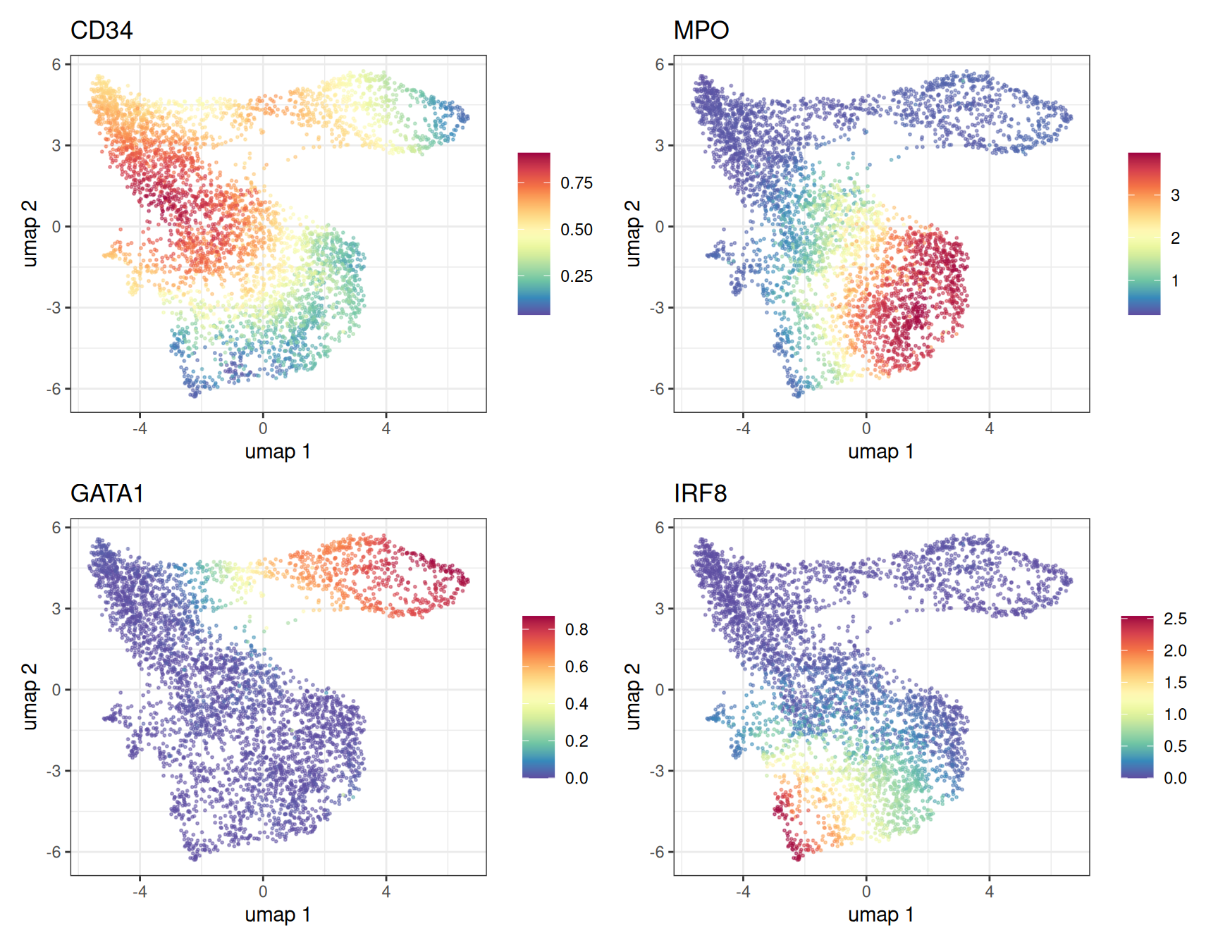
That is the picture people know from the paper, and it is worth being clear about what produced it. Neighbourhoods overlap, so smoothing over them makes nearby cells resemble each other in every gene at once. Gene-gene correlation after imputation is inflated, badly, and the inflation is a property of the graph rather than of the biology. Do not feed these values into Hotspot, SCENIC, differential correlation or CoReMo: those methods measure exactly the quantity MAGIC manufactures, and they will report the graph back to you as a finding. extract_dot_plot_data() has no layer argument for the same reason.
The layer is tracked like every other cached artefact, so it goes stale when the graph under it moves.
get_sc_cache_status(sc_object)
#>    modality  artefact   name stamped  stale reason               id
#>      <char>    <char> <char>  <lgcl> <lgcl> <char>           <char>
#> 1:      rna       pca   <NA>    TRUE  FALSE   <NA> 3f29eb1061f7bed7
#> 2:      rna embedding   umap    TRUE  FALSE   <NA> c35540cd15161d69
#> 3:      rna       knn   <NA>    TRUE  FALSE   <NA> f9b07f767ccf70a5
#> 4:      rna       snn   <NA>    TRUE  FALSE   <NA> 9f7436cb1c360def
#> 5:      rna     magic   <NA>    TRUE  FALSE   <NA> a1a1a95e6d4e5d57
#>                                 from
#>                               <list>
#> 1:
#> 2: 3f29eb1061f7bed7,f9b07f767ccf70a5
#> 3:                  3f29eb1061f7bed7
#> 4:                  f9b07f767ccf70a5
#> 5:                  f9b07f767ccf70a5
PAGA
PAGA is the cheap one, so start there. It reads the kNN indices and a clustering, ignores the distances entirely, and gives back a clusters-by-clusters graph.
paga_res <- run_paga_sc(
  sc_object,
  cluster_col = "leiden_clusters"
)
#> Running PAGA over the rna kNN graph (4142 cells, 8 clusters).
connectivities is the full abstracted graph, connectivities_tree its maximum spanning forest. Both are symmetric sparse matrices named by cluster, with a zero diagonal.
paga_res$sizes
#>    cluster n_cells
#>     <char>   <int>
#> 1:       0     693
#> 2:       1     669
#> 3:       2     618
#> 4:       3     555
#> 5:       4     531
#> 6:       5     486
#> 7:       6     444
#> 8:       7     146

round(as.matrix(paga_res$connectivities), 3)
#>       0     1     2     3     4     5     6     7
#> 0 0.000 0.490 0.001 0.001 0.001 0.016 0.006 0.400
#> 1 0.490 0.000 0.003 0.040 0.074 0.166 0.604 0.380
#> 2 0.001 0.003 0.000 0.004 0.004 0.003 0.014 0.349
#> 3 0.001 0.040 0.004 0.000 0.530 0.379 0.131 0.000
#> 4 0.001 0.074 0.004 0.530 0.000 0.036 0.412 0.001
#> 5 0.016 0.166 0.003 0.379 0.036 0.000 0.212 0.002
#> 6 0.006 0.604 0.014 0.131 0.412 0.212 0.000 0.036
#> 7 0.400 0.380 0.349 0.000 0.001 0.002 0.036 0.000
paga_plot_sc() puts every cluster at the centroid of its cells in an embedding and draws the graph over them. A free layout of the abstracted graph would put the nodes somewhere arbitrary, which you then have to relate back to the UMAP by eye.
paga_plot_sc(sc_object, paga_res, embedding = "umap")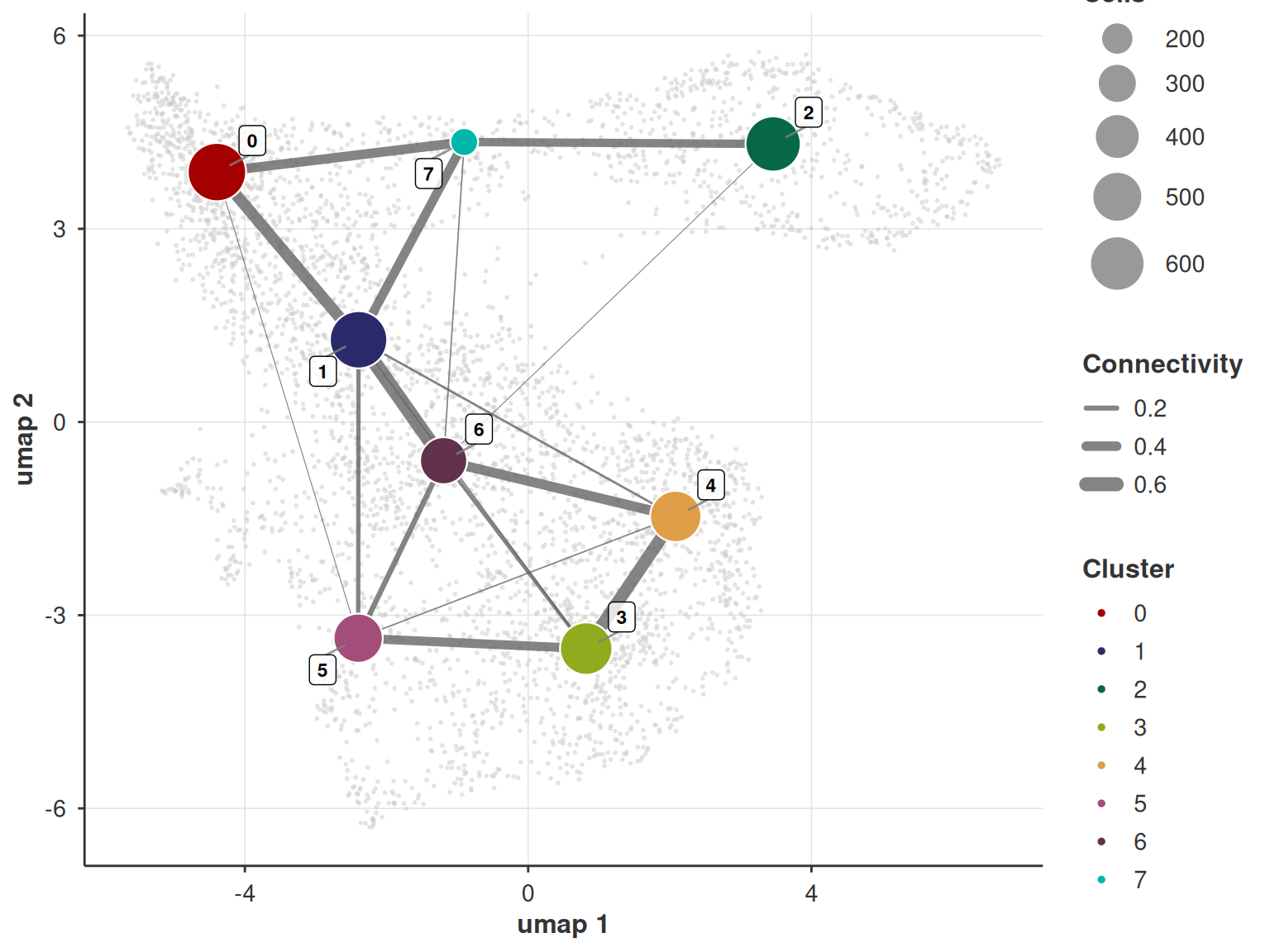
Edge thresholding is not optional. The abstracted graph is close to complete on real data, so at threshold = 0 you get a hairball. tree_only = TRUE is the shortcut to the backbone, and it is the readable one on anything above a handful of clusters.
paga_plot_sc(sc_object, paga_res, embedding = "umap", tree_only = TRUE)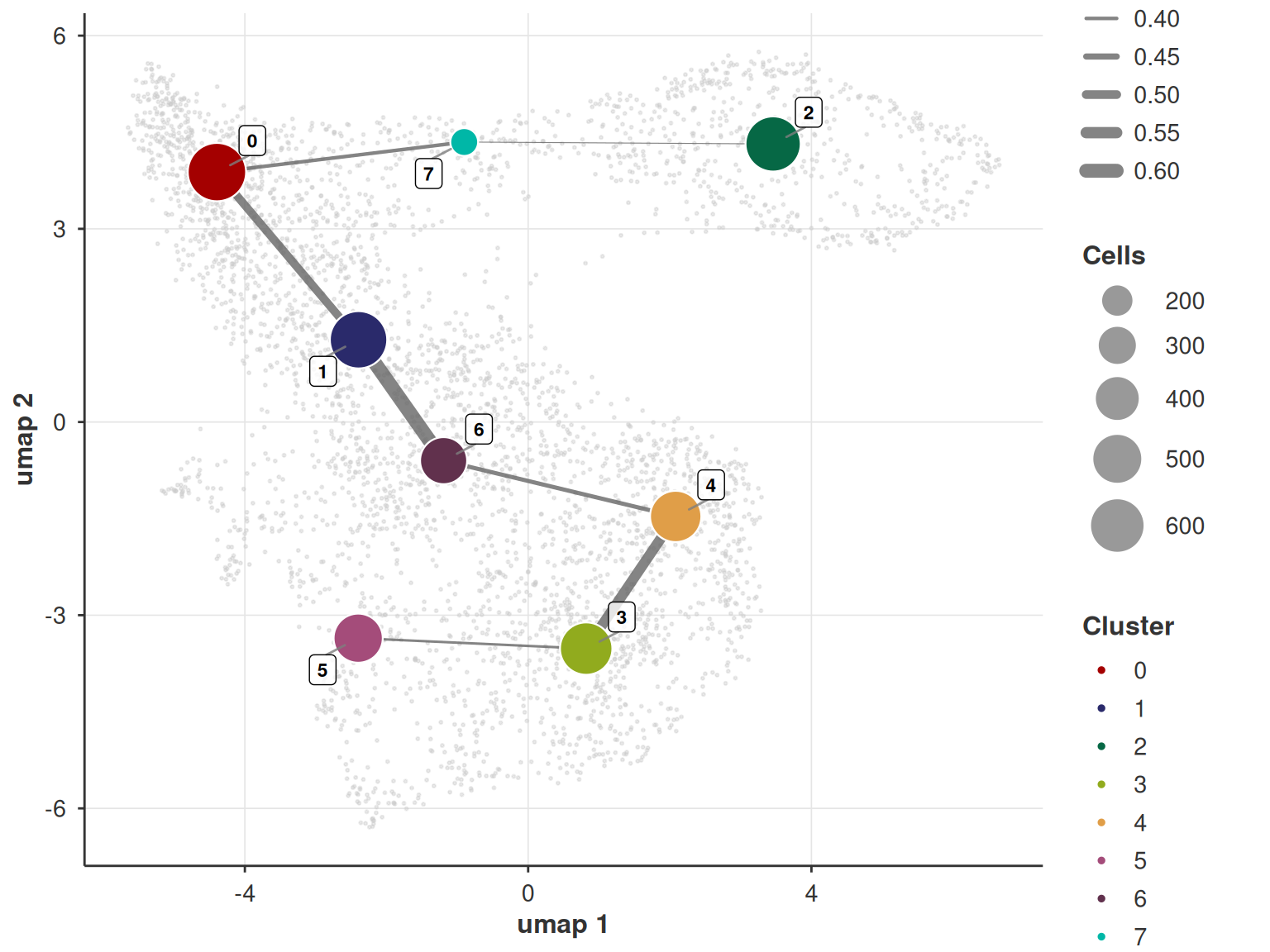
If you want the node and edge tables to draw yourself, they come out of extract_paga_plot_data(), which is what the plot is built on.
Palantir
The start cell and the three terminal states come straight from the reference notebook. The start cell was picked there for high CD34 expression; the terminal states are one cell each in the dendritic, monocyte and erythroid tips.
early_cell <- "Run5_164698952452459"

terminal_states <- c(
  DC = "Run5_131097901611291",
  Mono = "Run5_134936662236454",
  Ery = "Run4_200562869397916"
)
knn = 30 is the neighbour count for the geodesic graph Palantir builds on the multiscale space, a different knob from the k of the input kNN graph, and num_waypoints = 500 is the notebook’s override of the 1200 default.
Two things do not mirror the reference, and both change what you get.
use_early_cell_as_start is TRUE, so the early cell you name is the one that gets used. The reference snaps it to the nearest boundary cell of the diffusion map instead, and that candidate set is small, at most two cells per multiscale component. On a branching manifold the snap will cheerfully move a root cell onto a branch tip and run the whole trajectory backwards.
n_eigs is pinned at 10, leaving nine multiscale components. Left at NULL the count comes from the largest eigengap, which on this data picks 3, i.e. two components. Two components cannot resolve a three-way branch: the erythroid arm separates fine but the monocyte and dendritic fate probabilities end up correlated, their branch masks collapse onto each other, and the gene trends for those two lineages come out nearly identical. There is a section on that below.
palantir_res <- run_palantir_sc(
  sc_object,
  early_cell = early_cell,
  terminal_states = terminal_states,
  palantir_params = params_sc_palantir(
    n_eigs = 10L,
    knn = 30L
  ),
  seed = 42L
)
#> Running Palantir over the rna kNN graph (4142 cells).

palantir_res
#> PalantirRes: 4142 cells, 3 terminal states (rna modality)
#>   Start cell: Run5_164698952452459 | waypoints: 991
#>   Converged: TRUE (2 iterations)
#>   Repair edges: 0, stranded waypoints: 0
Two things to watch in that print out. repair_edges above zero means the kNN graph was disconnected and had to be bridged, which usually means k is too small for the data. A note about the diffusion eigensolve not converging means the embedding is under-resolved, and every distance taken on it is suspect; raise lanczos_max_restarts in params_sc_palantir() before believing anything downstream.
Results back onto the object
PalantirRes is keyed by cell name, not position, so match it against the obs cell names rather than assuming the two are in the same order.
obs_cells <- get_cell_names(sc_object, filtered = TRUE)
idx <- match(obs_cells, palantir_res$pseudotime$cell_id)

sc_object[["palantir_pseudotime"]] <- palantir_res$pseudotime$pseudotime[idx]
sc_object[["palantir_entropy"]] <- palantir_res$pseudotime$entropy[idx]
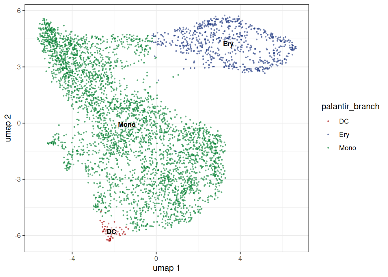
The fate probability matrix has one column per terminal state. Because terminal_states was a named vector, those names are already the column names, so all that is left is the dominant fate per cell.
fate_probs <- palantir_res$branch_probs[idx, ]

for (lineage in colnames(fate_probs)) {
  sc_object[[paste0("fate_", lineage)]] <- fate_probs[, lineage]
}

sc_object[["palantir_branch"]] <- colnames(fate_probs)[
  max.col(fate_probs, ties.method = "first")
]

head(round(fate_probs, 3))
#>                        Ery    DC  Mono
#> Run4_120703408880541 0.634 0.067 0.299
#> Run4_120703409056541 0.284 0.132 0.585
#> Run4_120703409580963 0.075 0.129 0.797
#> Run4_120703423990708 0.012 0.019 0.969
#> Run4_120703436876077 0.269 0.134 0.597
#> Run4_120726912355038 0.153 0.136 0.711
Rows do not necessarily sum to one. Fate probabilities below branch_prob_threshold (0.01 by default) are zeroed without renormalisation, and cells whose waypoint weight sits on a stranded waypoint lose that mass entirely.
Pseudotime and entropy
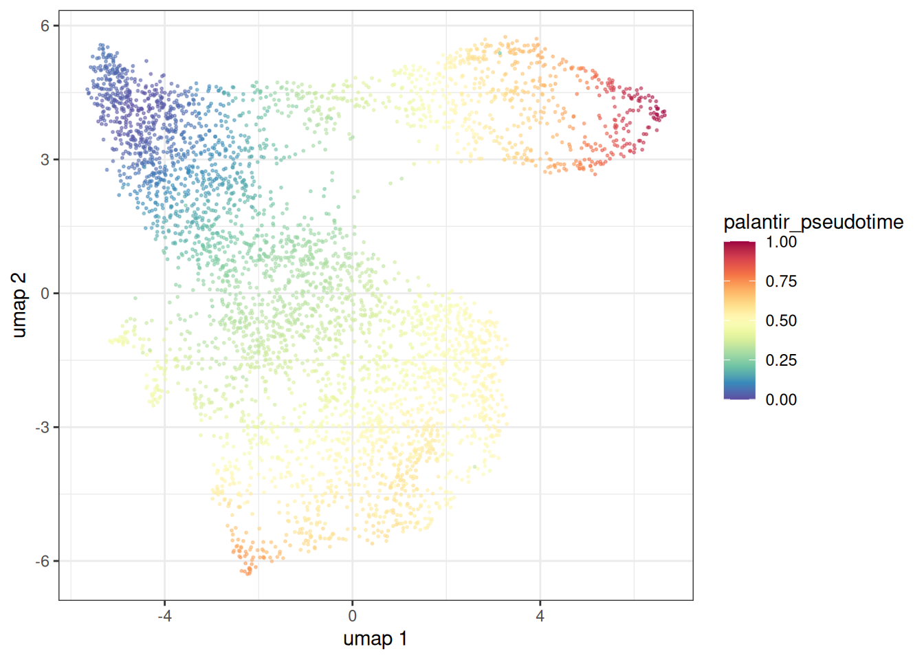
embedding_plot_sc(
  sc_object,
  embedding = "umap",
  colour_by = "palantir_pseudotime",
  palette = "spectral",
  discrete = FALSE
)
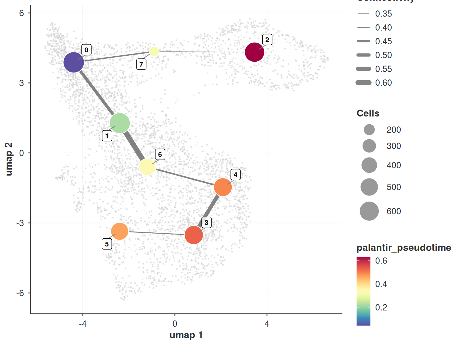
The same quantity on the abstracted graph is worth a look, because it is the cheapest check that the two methods agree. PAGA knows nothing about pseudotime, so if its backbone and the pseudotime gradient point in different directions, one of them is wrong.
paga_plot_sc(
  sc_object,
  paga_res,
  embedding = "umap",
  node_colour_by = "palantir_pseudotime",
  palette = "spectral",
  tree_only = TRUE
)
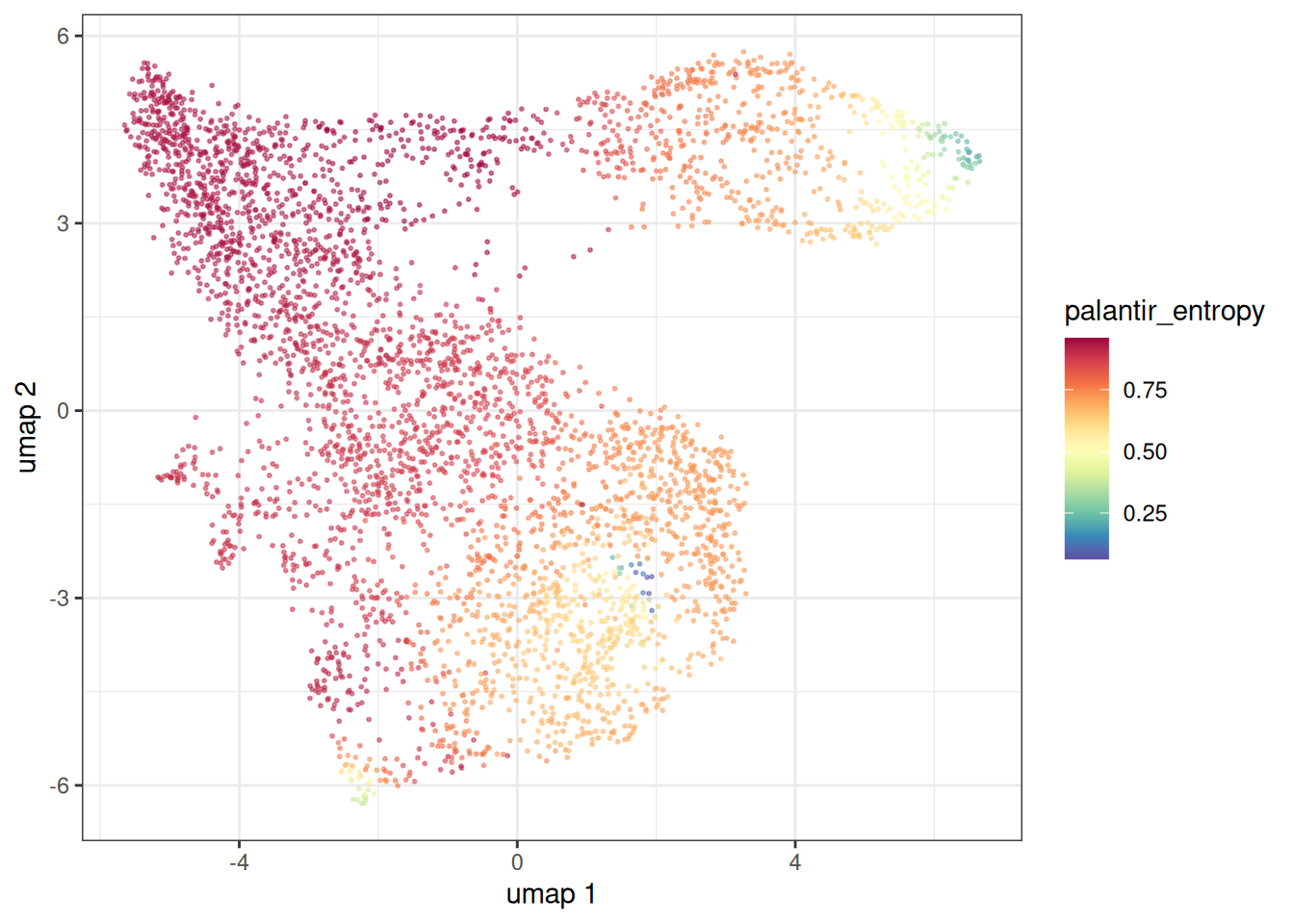
Entropy is high where a cell still has several fates open to it and drops to zero once it commits. On a clean three-lineage data set the stem pool should sit near log(3).
embedding_plot_sc(
  sc_object,
  embedding = "umap",
  colour_by = "palantir_entropy",
  palette = "spectral",
  discrete = FALSE
)
fate_plots <- lapply(colnames(fate_probs), \(lineage) {
  embedding_plot_sc(
    sc_object,
    embedding = "umap",
    colour_by = paste0("fate_", lineage),
    palette = "spectral",
    discrete = FALSE
  ) +
    labs(title = lineage)
})

wrap_plots(fate_plots, nrow = 1)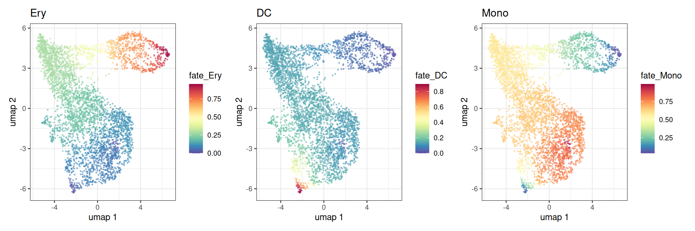
embedding_plot_sc(
  sc_object,
  embedding = "umap",
  colour_by = "palantir_branch",
  label_by = "palantir_branch",
  discrete = TRUE
)
Letting Palantir find the terminal states
Drop terminal_states and they get detected from the waypoint Markov chain instead. Handy when you have no prior, but treat the result as a starting point rather than an answer: the detection reads extremes of the multiscale space, and on data sets this size those are not always well determined.
palantir_auto <- run_palantir_sc(
  sc_object,
  early_cell = early_cell,
  palantir_params = params_sc_palantir(
    n_eigs = 10L,
    knn = 30L,
    use_early_cell_as_start = TRUE
  ),
  seed = 42L
)
#> Running Palantir over the rna kNN graph (4142 cells).

palantir_auto$terminal_states
#> [1] "Run5_134377557125406"
Where did they land relative to the supplied ones?
data.table(
  cell_id = palantir_auto$terminal_states,
  branch = unlist(sc_object[["palantir_branch"]], use.names = FALSE)[
    match(palantir_auto$terminal_states, obs_cells)
  ],
  pseudotime = round(
    palantir_res$pseudotime$pseudotime[
      match(palantir_auto$terminal_states, palantir_res$pseudotime$cell_id)
    ],
    3
  )
)
#>                 cell_id branch pseudotime
#>                  <char> <char>      <num>
#> 1: Run5_134377557125406   Mono      0.324
Gene trends
run_gene_trends_sc() does two things. First it assigns cells to branches: for each fate, the probability threshold is an expanding quantile over the pseudotime-sorted cells, made monotone with a cumulative maximum, so a fate’s bar can only rise as differentiation proceeds. Then it fits a landmark Gaussian process with a Matern-5/2 kernel per branch, on a 500 point pseudotime grid.
trends <- run_gene_trends_sc(
  sc_object,
  palantir_res = palantir_res,
  features = markers
)
#> Fitting gene trends over 3 branches (4142 cells, 4 genes, normalised counts).

trends
#> GeneTrendsRes: 3 branches, 4 genes, 500 grid points
#>   Cells per branch: Ery (1425), DC (1532), Mono (1981)
#>   Source: normalised counts
#>   Length scale: 1 | sigma: 1
trends$trends is a long data.table with branch, pseudotime, gene and expression, which is what a facet wants.
ggplot(
  trends$trends,
  aes(x = pseudotime, y = expression, colour = branch)
) +
  geom_line(linewidth = 0.8) +
  facet_wrap(~gene, scales = "free_y") +
  scale_color_bx() +
  labs(
    x = "Palantir pseudotime",
    y = "Normalised expression",
    colour = "Lineage"
  ) +
  theme_bx()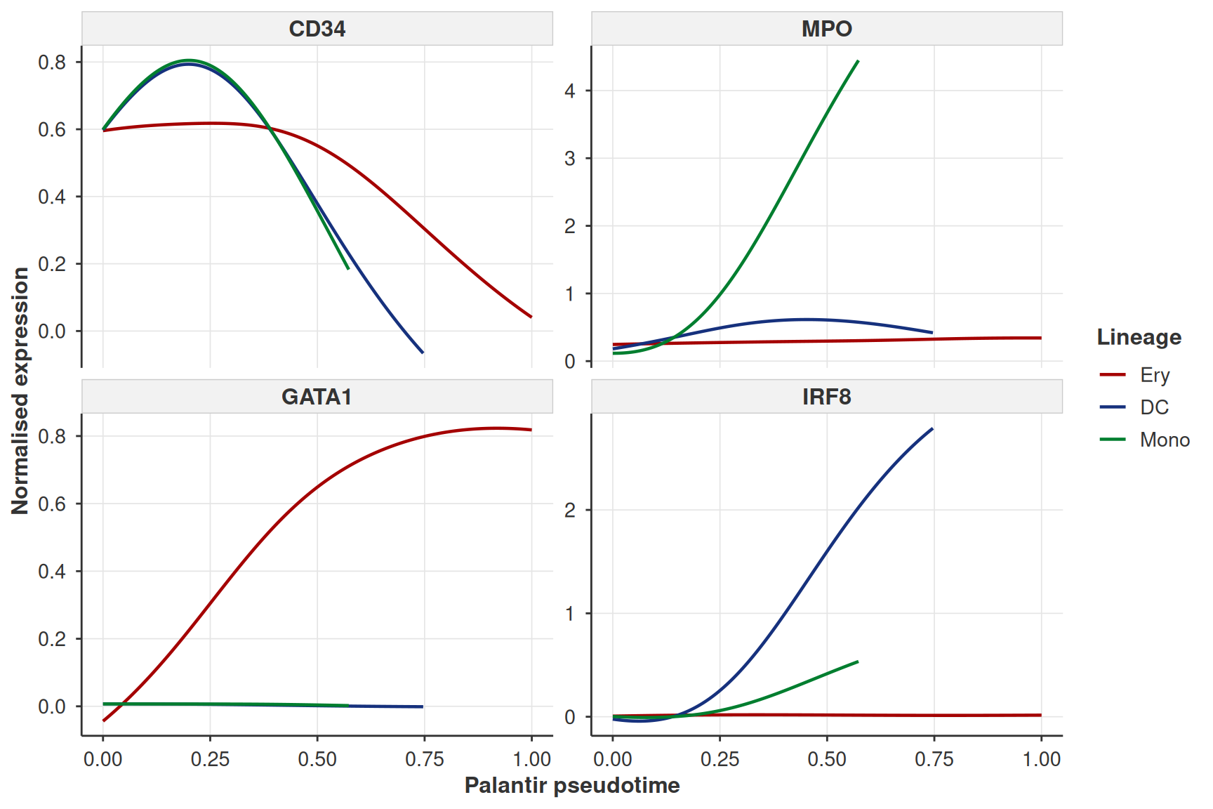
CD34 falls away from the root, GATA1 climbs on the erythroid arm, MPO on the monocyte one, IRF8 on the dendritic one. Set use_magic = TRUE to fit the imputed layer instead, which is what the reference notebook does. Note that the GP already smooths over pseudotime, so imputing first smooths twice.
branch_cells carries the selection itself, which is the branch cell set the reference notebook plots.
purrr::map_int(trends$branch_cells, length)
#>  Ery   DC Mono
#> 1425 1532 1981
The same trick works with any per-cell quantity. A loess through the entropy column watches commitment happen along the trajectory.
obs_dt <- get_sc_obs(sc_object, filtered = TRUE)

ggplot(
  obs_dt,
  aes(x = palantir_pseudotime, y = palantir_entropy, colour = palantir_branch)
) +
  geom_point(size = 0.4, alpha = 0.3) +
  geom_smooth(method = "loess", formula = y ~ x, se = FALSE, span = 0.6) +
  scale_color_bx() +
  labs(
    x = "Palantir pseudotime",
    y = "Differentiation entropy",
    colour = "Dominant fate"
  ) +
  theme_bx()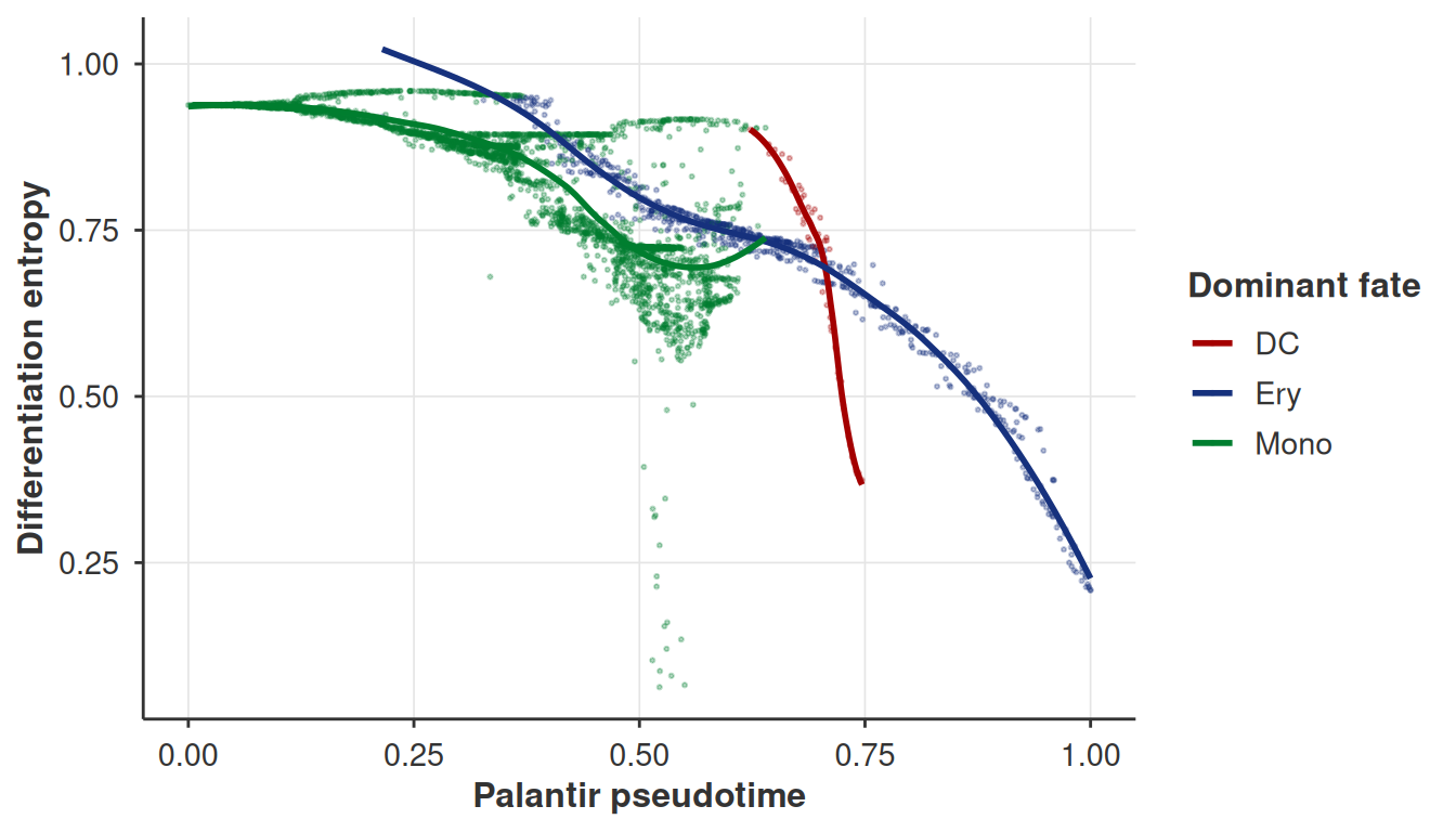
Where this can go wrong
Palantir has more moving parts than most methods in this package, and several of them fail quietly rather than loudly. In rough order of how often they bite:
-
pruningleft at its default. Covered above, and the only one on this list that is upstream of Palantir entirely. It costs you clusters, not pseudotime, but a one-cell cluster then walks into PAGA and comes back out as a fat edge into a dot, because the null model has almost no possible edges to normalise against. -
The start cell. Covered above. Set
use_early_cell_as_start = FALSEto get the reference behaviour and it can move your root onto a branch tip. If pseudotime comes back anti-correlated with what you expect, checkstart_cellon the result object first. Note that pseudotime is not pinned to zero at the start cell either: the refinement can put the minimum on a neighbour, and a start cell far from zero means it disagreed with your anchor. -
eigen_converged = FALSE. The diffusion eigensolve ran out of restarts, so the multiscale embedding is under-resolved. Everything downstream converges happily on noise, which is exactly why this is reported. Raiselanczos_max_restarts. -
repair_edges > 0. The kNN graph was disconnected and Palantir bridged it to carry on. Raisekonfind_neighbours_sc()rather than living with the bridges. -
stranded_waypoints > 0. Waypoints from which no terminal state is reachable. Their cells lose fate probability mass, so rows sum below one. A large count means the pseudotime-directed pruning cut too hard. -
n_eigs. The one that bites hardest, and it is silent. Left atNULLthe eigenvector count comes from the largest eigengap, which on this data picks 3, leaving two multiscale components for a three-way branch. Nothing errors. What happens instead is that two of the three fates stop separating: their probabilities correlate,select_branch_cells()hands the two branches almost the same cells, and their gene trends come out on top of each other. Here the monocyte and dendritic masks shared 80% of their cells at the default, with exactly one cell unique to the monocyte branch, and pinningn_eigsto 10 is what fixes it. If two lineages give you the same curve, count the components before you blame the estimator. -
Branch masks are permissive by design. Even at a sensible
n_eigs, a cell belongs to a branch when its fate probability is near the top of what has been seen up to its pseudotime, so the uncommitted trunk sits in every branch at once. That is the reference’s logic and it is the right one, but it means two branches only diverge where their late cells differ. Checkbranch_cellsoverlap before reading much into two curves that hug. -
The gene trend defaults are prior-dominated. Pseudotime is min-max scaled to
[0, 1], so the reference’slength_scale = 1spans the entire domain and itssigma = 1sits at roughly the signal scale of log-normalised expression. Almost any gene resolves into a smooth monotone or single-peaked curve. That is a presentation choice, not inference. Shortenlength_scaleinparams_sc_gene_trends()before believing a bump. -
Double smoothing. MAGIC averages over the graph and the GP averages over pseudotime. Running both is defensible for a figure and rarely necessary for the trend itself. If a feature only shows up with
use_magic = TRUE, that is worth knowing about it. -
A stale imputed layer. The layer is stamped against the kNN graph it came from, so
get_sc_cache_status()flags it once the graph or the cell filter moves.run_gene_trends_sc(use_magic = TRUE)refuses to fit a stale one.