
Ligand-receptor analysis with bixverse
2026-10-27
Intro
This vignette runs two flavours of ligand-receptor analysis on the PBMC3k data set. It assumes you know your way around the SingleCells class and the basic processing pipeline. If not, have a look at the PBMC processing vignette first.
The two approaches answer different questions:
- CellPhoneDB asks which ligand-receptor pairs are expressed between two cell types, more so than you’d expect by chance. It works off expression alone, handles multi-subunit receptor complexes and comes with a curated database of ~2,900 interactions.
- NicheNet goes one step further and asks which ligands best explain a downstream transcriptional response in the receiver. That needs a signalling and a gene regulatory network on top.
Both share the processing and the marker genes, so we do that once.
Loading and processing PBMC3k
We reuse the standard processing pipeline. See the PBMC processing vignette for commentary on each step.
pbmc3k_path <- download_pbmc3k()
tempdir_pbmc <- tempdir()

sc_object <- SingleCells(dir_data = tempdir_pbmc)
mtx_io_params <- get_cell_ranger_params(pbmc3k_path)

sc_object <- load_mtx(
  object = sc_object,
  sc_mtx_io_param = mtx_io_params,
  mtx_streaming = FALSE,
  .verbose = FALSE
)

setnames_sc(sc_object, table = "var", old = "column1", new = "gene_symbol")
var <- get_sc_var(sc_object)
symbol_to_ensembl <- setNames(var$gene_id, var$gene_symbol)
ensembl_to_symbol <- setNames(var$gene_symbol, var$gene_id)

# QC and processing
gs_of_interest <- list(
  MT = var[grepl("^MT-", gene_symbol), gene_id],
  Ribo = var[grepl("^RPS|^RPL", gene_symbol), gene_id]
)
sc_object <- gene_set_proportions_sc(
  sc_object,
  gs_of_interest,
  .verbose = FALSE
)

# minimal cell filtering
cells_to_keep <- sc_object[[]][MT < 0.2, cell_id]
sc_object <- set_cells_to_keep(sc_object, cells_to_keep)

sc_object <- find_hvg_sc(sc_object, hvg_no = 2000L, .verbose = FALSE)
sc_object <- calculate_pca_sc(sc_object, no_pcs = 30L, .verbose = FALSE)
sc_object <- find_neighbours_sc(sc_object, .verbose = FALSE)
sc_object <- find_clusters_sc(sc_object, res = 0.5)
For demonstration purposes we use the Leiden cluster IDs directly as cell types. In a real analysis you’d annotate the clusters first (marker genes, a canonical panel, assign_sc_type(), take your pick). Senders and receivers are biological concepts, and “cluster_3 talks to cluster_0” doesn’t tell anyone much.
sc_object[["celltype"]] <- paste0(
  "cluster_",
  unlist(sc_object[["leiden_clustering"]])
)

celltype_counts <- sc_object[[]][!is.na(celltype), .N, by = celltype][order(-N)]

celltype_counts
#>     celltype     N
#>       <char> <int>
#> 1: cluster_0  1194
#> 2: cluster_1   490
#> 3: cluster_2   459
#> 4: cluster_3   346
#> 5: cluster_4   164
#> 6: cluster_5    32
#> 7: cluster_6    13
Both methods want per-cluster marker genes, so let’s get them out of the way. find_all_markers_sc() runs a one-vs-rest Wilcoxon test per cluster.
celltype_de <- find_all_markers_sc(
  object = sc_object,
  column_of_interest = "celltype",
  .verbose = FALSE
)

# rename to the schema the downstream functions expect
setnames(
  celltype_de,
  c("gene_id", "grp", "p_values"),
  c("gene", "cluster_id", "pval"),
  skip_absent = TRUE
)
CellPhoneDB
The database
get_cellphonedb_db() pulls the CellPhoneDB v5 database and flattens it to one row per interaction. Each partner comes with the gene symbols of its subunits: one gene for a plain protein, several for a complex.
cpdb_db <- get_cellphonedb_db(dir = tempdir_pbmc, .verbose = FALSE)

cpdb_db[, .N, by = directionality]
#>       directionality     N
#>               <char> <int>
#> 1:   Ligand-Receptor  2508
#> 2: Receptor-Receptor    28
#> 3: Adhesion-Adhesion   242
#> 4:     Ligand-Ligand   123
#> 5:           Gap-Gap    10
A few receptors are complexes, e.g. the TGF-beta receptors:
cpdb_db[partner_a == "TGFB1", .(partner_a, partner_b, genes_b)]
#>    partner_a             partner_b       genes_b
#>       <char>                <char>        <list>
#> 1:     TGFB1     TGFbeta_receptor2  ACVR1,TGFBR2
#> 2:     TGFB1 integrin_aVb6_complex   ITGAV,ITGB6
#> 3:     TGFB1     TGFbeta_receptor1 TGFBR1,TGFBR2
#> 4:     TGFB1                TGFBR3        TGFBR3
Got your own curated list? Any data.table with interaction_id, partner_a, partner_b and the list columns genes_a and genes_b works.
Statistical analysis
For every interaction and every ordered (sender, receiver) cluster pair, partner a is measured in the sender and partner b in the receiver. The interaction mean is the average of the two partner means, and a complex takes the minimum over its subunits. Both partners need to be expressed in more than 10% of their cluster’s cells (the gate). The p-value comes from shuffling the cluster labels 1,000 times. The database speaks gene symbols, so we point gene_id_col at the symbol column.
cpdb_res <- cellphonedb_sc(
  object = sc_object,
  celltype_colname = "celltype",
  lr_db = cpdb_db,
  gene_id_col = "gene_symbol",
  params = params_sc_cellphonedb(n_perm = 1000L)
)
#> Warning in cellphonedb_sc(object = sc_object, celltype_colname = "celltype", :
#> Dropping 2753 of 2911 interactions with subunits missing from `object`.

cpdb_sig <- cpdb_res[gate == TRUE & pval <= 0.05]

nrow(cpdb_sig)
#> [1] 320
That’s a lot of dropped interactions. load_mtx() throws out genes seen in fewer than 10 cells, and much of CellPhoneDB (neurotransmitter transporters, neuronal receptors, …) is simply not expressed in blood:
An interaction needs every subunit of both partners, which leaves 158 interactions to test.
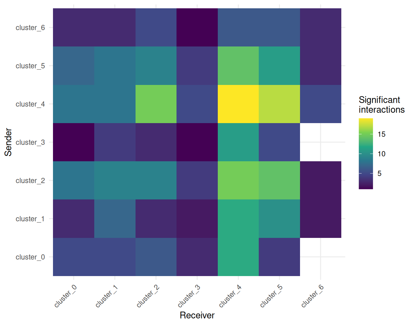
Which cluster pairs talk the most? Counting the significant interactions per pair gives the classic CellPhoneDB heatmap.
pair_counts <- cpdb_sig[, .N, by = .(sender, receiver)]

ggplot(pair_counts, aes(x = receiver, y = sender, fill = N)) +
  geom_tile() +
  scale_fill_viridis_c() +
  theme_minimal() +
  theme(axis.text.x = element_text(angle = 45, hjust = 1)) +
  labs(
    x = "Receiver",
    y = "Sender",
    fill = "Significant\ninteractions"
  )
And the strongest interactions by mean:
head(
  cpdb_sig[order(-mean), .(sender, receiver, partner_a, partner_b, mean, pval)],
  10
)
#>        sender  receiver partner_a partner_b     mean  pval
#>        <char>    <char>    <char>    <char>    <num> <num>
#>  1: cluster_6 cluster_5       APP      CD74 2.982131     0
#>  2: cluster_6 cluster_3       APP      CD74 2.918462     0
#>  3: cluster_5 cluster_5       APP      CD74 2.685051     0
#>  4: cluster_6 cluster_5       PF4     CXCR3 2.648153     0
#>  5: cluster_5 cluster_3       APP      CD74 2.621382     0
#>  6: cluster_4 cluster_1      CD44    TYROBP 2.550512     0
#>  7: cluster_4 cluster_4      CD44    TYROBP 2.454405     0
#>  8: cluster_0 cluster_1      CD44    TYROBP 2.405280     0
#>  9: cluster_1 cluster_1      CD44    TYROBP 2.369329     0
#> 10: cluster_0 cluster_4      CD44    TYROBP 2.309173     0
Two things to keep in mind here. First, the permutation test asks for specificity, not just expression. PPIA-BSG passes the expression gate in 49 of the 49 cluster pairs, but is significant in only 20 of them. Second, the top of that list is dominated by clusters 6 to 8, which hold 13 cells. Means over a handful of cells are noisy, so treat hits from tiny clusters with care.
DEG-based analysis
The alternative is CellPhoneDB’s DEG-based method. No permutations here. Instead, an interaction is kept for a pair if the expression gate passes and partner a is a marker of the sender or partner b a marker of the receiver. You decide what counts as a marker. Here we take genes with a log fold change above 0.5 and FDR <= 0.05, and convert them to symbols to match the database.
deg_table <- celltype_de[lfc > 0.5 & fdr <= 0.05, .(cluster_id, gene)]
deg_table[, gene := ensembl_to_symbol[gene]]

cpdb_deg_res <- suppressWarnings(cellphonedb_sc(
  object = sc_object,
  celltype_colname = "celltype",
  lr_db = cpdb_db,
  method = "degs",
  deg_table = deg_table,
  gene_id_col = "gene_symbol"
))

cpdb_relevant <- cpdb_deg_res[gate == TRUE]

head(
  cpdb_relevant[order(-mean), .(sender, receiver, partner_a, partner_b, mean)],
  10
)
#>        sender  receiver partner_a partner_b     mean
#>        <char>    <char>    <char>    <char>    <num>
#>  1: cluster_6 cluster_5       APP      CD74 2.982131
#>  2: cluster_6 cluster_3       APP      CD74 2.918462
#>  3: cluster_5 cluster_5       APP      CD74 2.685051
#>  4: cluster_6 cluster_5       PF4     CXCR3 2.648153
#>  5: cluster_5 cluster_3       APP      CD74 2.621382
#>  6: cluster_4 cluster_1      CD44    TYROBP 2.550512
#>  7: cluster_4 cluster_4      CD44    TYROBP 2.454405
#>  8: cluster_0 cluster_1      CD44    TYROBP 2.405280
#>  9: cluster_1 cluster_1      CD44    TYROBP 2.369329
#> 10: cluster_0 cluster_4      CD44    TYROBP 2.309173
181 interaction and cluster pair combinations pass the DEG gate, and 162 of them are also significant in the permutation run. This is the route to take if you’ve got a proper DE setup, e.g. pseudo-bulk across samples (see the notes at the end). The cell type specificity then comes from the DE test instead of from shuffling labels.
NicheNet
NicheNet ranks upstream ligands by how well their predicted target genes line up with a gene set of interest in a receiver cell type. The pipeline:
- Build a ligand-target regulatory potential matrix from a signalling network (PPI) and a gene regulatory network (GRN).
- Define a gene set of interest in the receiver (here, its marker genes).
- Score each ligand by how well its targets overlap with that gene set (AUROC, AUPR, correlations).
- Combine ligand activity with sender/receiver expression and DE into a single prioritisation score.
Building the networks
A production analysis would load the curated NicheNet networks (signalling and GRN) from Zenodo. To keep the vignette self-contained, we construct a small network covering a handful of canonical immune signalling pathways. The shape of the inputs is what matters here… and it means you can feed in your own networks.
# Ligand-receptor pairs (canonical immune signalling)
lr_network <- data.table(
  # ligands
  from = c("CCL5", "CXCL10", "IL15", "TNF", "TGFB1", "IL10", "ICAM1"),
  # receptors
  to = c(
    "CCR5",
    "CXCR3",
    "IL2RG",
    "TNFRSF1A",
    "TGFBR2",
    "IL10RA",
    "ITGAL"
  ),
  weight = 1
)

# Signalling (PPI) layer: ligand -> receptor -> intracellular signalling -> TFs
ppi_network <- data.table(
  from = c(
    "CCL5",
    "CXCL10",
    "IL15",
    "TNF",
    "TGFB1",
    "IL10",
    "ICAM1",
    "CCR5",
    "CXCR3",
    "IL2RG",
    "TNFRSF1A",
    "TGFBR2",
    "IL10RA",
    "ITGAL",
    "JAK1",
    "JAK2",
    "JAK3",
    "STAT1",
    "STAT3",
    "STAT5A",
    "NFKB1",
    "SMAD2"
  ),
  to = c(
    "CCR5",
    "CXCR3",
    "IL2RG",
    "TNFRSF1A",
    "TGFBR2",
    "IL10RA",
    "ITGAL",
    "JAK1",
    "JAK1",
    "JAK3",
    "NFKB1",
    "SMAD2",
    "JAK1",
    "NFKB1",
    "STAT1",
    "STAT3",
    "STAT5A",
    "STAT3",
    "STAT1",
    "STAT3",
    "STAT3",
    "STAT3"
  ),
  weight = 1
)

# GRN layer: TF -> targets
grn_network <- data.table(
  from = c(
    rep("STAT1", 6),
    rep("STAT3", 6),
    rep("STAT5A", 4),
    rep("NFKB1", 6),
    rep("SMAD2", 4)
  ),
  to = c(
    "IRF1",
    "MX1",
    "ISG15",
    "OAS1",
    "GBP1",
    "CXCL10",
    "SOCS3",
    "IL6",
    "BCL2",
    "VEGFA",
    "MYC",
    "FOS",
    "CCND1",
    "BCL2L1",
    "IL2RA",
    "FOXP3",
    "TNF",
    "IL1B",
    "IL6",
    "NFKBIA",
    "CCL5",
    "ICAM1",
    "SERPINE1",
    "CDKN1A",
    "JUNB",
    "ID1"
  ),
  weight = 1
)
Map gene symbols to the Ensembl IDs used internally by sc_object, dropping any genes not present in the data set.
symbol_to_id <- function(syms) {
  ids <- symbol_to_ensembl[syms]
  ids[!is.na(ids)]
}

# Restrict the networks to genes present in PBMC3k
keep_ppi <- ppi_network$from %in%
  names(symbol_to_ensembl) &
  ppi_network$to %in% names(symbol_to_ensembl)
keep_grn <- grn_network$from %in%
  names(symbol_to_ensembl) &
  grn_network$to %in% names(symbol_to_ensembl)
keep_lr <- lr_network$from %in%
  names(symbol_to_ensembl) &
  lr_network$to %in% names(symbol_to_ensembl)

ppi_network <- ppi_network[keep_ppi]
grn_network <- grn_network[keep_grn]
lr_network <- lr_network[keep_lr]
Ligand-target regulatory potential
Construct the ligand-target influence matrix. Each row is one ligand and each column is a gene from the union of both networks; entries are NicheNet-style regulatory potential scores.
ligand_seeds <- setNames(
  lapply(lr_network$from, identity),
  lr_network$from
)

ligand_influence <- generate_ligand_target_influence(
  ligand_seeds = ligand_seeds,
  ppi_network = rbind(lr_network, ppi_network),
  grn_network = grn_network,
  # because of the tiny network, the original ltf_cutoff of 0.99 would be way
  # too aggressive
  params = params_ligand_target(ltf_cutoff = 0)
)

ligand_influence
#> LigandTargetInfluence
#>   No ligand seeds:    6
#>   No genes:           40
#>   Damping factor:     0.500
#>   Max iter:           1000
#>   Secondary targets:  FALSE
This returns a LigandTargetInfluence class. If you want to access the actual scores, you can use:
get_influence(ligand_influence)
#>         CCL5     CXCL10 IL15   TNF TGFB1 ICAM1 CCR5 CXCR3 IL2RG TNFRSF1A TGFBR2
#> CCL5   0.000 0.08333333    0 0.000     0 0.000    0     0     0        0      0
#> CXCL10 0.000 0.08333333    0 0.000     0 0.000    0     0     0        0      0
#> IL15   0.000 0.02083333    0 0.000     0 0.000    0     0     0        0      0
#> TNF    0.125 0.04166667    0 0.125     0 0.125    0     0     0        0      0
#> TGFB1  0.000 0.04166667    0 0.000     0 0.000    0     0     0        0      0
#> ICAM1  0.125 0.04166667    0 0.125     0 0.125    0     0     0        0      0
#>        IL10RA ITGAL JAK1 JAK2 JAK3 STAT1 STAT3 STAT5A NFKB1 SMAD2       IRF1
#> CCL5        0     0    0    0    0     0     0      0     0     0 0.08333333
#> CXCL10      0     0    0    0    0     0     0      0     0     0 0.08333333
#> IL15        0     0    0    0    0     0     0      0     0     0 0.02083333
#> TNF         0     0    0    0    0     0     0      0     0     0 0.04166667
#> TGFB1       0     0    0    0    0     0     0      0     0     0 0.04166667
#> ICAM1       0     0    0    0    0     0     0      0     0     0 0.04166667
#>               MX1      ISG15       OAS1       GBP1      SOCS3        IL6
#> CCL5   0.08333333 0.08333333 0.08333333 0.08333333 0.04166667 0.04166667
#> CXCL10 0.08333333 0.08333333 0.08333333 0.08333333 0.04166667 0.04166667
#> IL15   0.02083333 0.02083333 0.02083333 0.02083333 0.04166667 0.04166667
#> TNF    0.04166667 0.04166667 0.04166667 0.04166667 0.08333333 0.20833333
#> TGFB1  0.04166667 0.04166667 0.04166667 0.04166667 0.08333333 0.08333333
#> ICAM1  0.04166667 0.04166667 0.04166667 0.04166667 0.08333333 0.20833333
#>              BCL2      VEGFA        MYC        FOS BCL2L1  IL2RA  FOXP3  IL1B
#> CCL5   0.04166667 0.04166667 0.04166667 0.04166667 0.0000 0.0000 0.0000 0.000
#> CXCL10 0.04166667 0.04166667 0.04166667 0.04166667 0.0000 0.0000 0.0000 0.000
#> IL15   0.04166667 0.04166667 0.04166667 0.04166667 0.0625 0.0625 0.0625 0.000
#> TNF    0.08333333 0.08333333 0.08333333 0.08333333 0.0000 0.0000 0.0000 0.125
#> TGFB1  0.08333333 0.08333333 0.08333333 0.08333333 0.0000 0.0000 0.0000 0.000
#> ICAM1  0.08333333 0.08333333 0.08333333 0.08333333 0.0000 0.0000 0.0000 0.125
#>        NFKBIA CDKN1A  JUNB   ID1
#> CCL5    0.000  0.000 0.000 0.000
#> CXCL10  0.000  0.000 0.000 0.000
#> IL15    0.000  0.000 0.000 0.000
#> TNF     0.125  0.000 0.000 0.000
#> TGFB1   0.000  0.125 0.125 0.125
#> ICAM1   0.125  0.000 0.000 0.000
Defining the gene set of interest
In a case/control experiment, the gene set of interest would be the DEGs between conditions in the receiver cell type. PBMC3k is a single condition, so we use the receiver’s markers as a stand-in. We pick the largest cluster as receiver and a few others as senders.
Ligand activity scoring
Score each ligand by how well its target potential vector aligns with geneset_oi. The background is the full set of genes in the influence matrix.
activity <- ligand_activity_scores(
  ligand_influence = ligand_influence,
  # need to transform to gene symbols
  gene_sets = list(receiver_degs = ensembl_to_symbol[geneset_oi])
)

activity[order(-aupr_corrected)]
#>         gene_set ligand     auroc      aupr aupr_corrected      pearson
#>           <char> <char>     <num>     <num>          <num>        <num>
#> 1: receiver_degs  TGFB1 0.6594982 0.3956790    0.170679012  0.299473381
#> 2: receiver_degs   IL15 0.5663082 0.2353395    0.010339506  0.117053047
#> 3: receiver_degs   CCL5 0.5501792 0.2291667    0.004166667 -0.004045534
#> 4: receiver_degs CXCL10 0.5501792 0.2291667    0.004166667 -0.004045534
#> 5: receiver_degs    TNF 0.5125448 0.2086676   -0.016332442 -0.004747876
#> 6: receiver_degs  ICAM1 0.5125448 0.2086676   -0.016332442 -0.004747876
#>      spearman
#>         <num>
#> 1: 0.26664795
#> 2: 0.11085364
#> 3: 0.09001531
#> 4: 0.09001531
#> 5: 0.02025577
#> 6: 0.02025577
Sender and receiver tables
Prioritisation needs the DE of ligands across senders and of receptors in the receiver (we’ve got that from the markers), plus the average expression of ligands and receptors per cluster. The latter calls into the streaming engine via compute_expression_info_sc().
genes_of_interest <- union(lr_network$to, lr_network$from)
genes_of_interest_ids <- symbol_to_id(genes_of_interest)

expression_info <- compute_expression_info_sc(
  object = sc_object,
  celltype_colname = "celltype",
  genes = genes_of_interest_ids
)
Prioritisation
Combine all of the above into a single weighted score. PBMC3k has no condition contrast, so we use the "one_condition" scenario, which sets the condition-specificity weights to zero.
# Reduce activity table to one row per ligand (we ran one gene set)
la_input <- activity[, .(ligand, aupr_corrected)]
la_input[, ligand := symbol_to_ensembl[ligand]]

lr_network_ensembl <- data.table(
  ligand = symbol_to_ensembl[lr_network$from],
  receptor = symbol_to_ensembl[lr_network$to]
) %>%
  na.omit()

result <- prioritise_interactions(
  celltype_de = celltype_de[, .(cluster_id, gene, lfc, pval)],
  expression_info = expression_info,
  ligand_activities = na.omit(la_input),
  lr_network = lr_network_ensembl,
  senders_oi = senders_oi,
  receivers_oi = receiver_id,
  scenario = "one_condition"
)
Add symbol columns for readability.
result[, ligand_symbol := ensembl_to_symbol[ligand]]
result[, receptor_symbol := ensembl_to_symbol[receptor]]

head(
  result[, .(
    sender,
    receiver,
    ligand_symbol,
    receptor_symbol,
    prioritisation_score,
    prioritisation_rank
  )],
  10
)
#>       sender  receiver ligand_symbol receptor_symbol prioritisation_score
#>       <char>    <char>        <char>          <char>                <num>
#> 1: cluster_4 cluster_0         TGFB1          TGFBR2            0.8333333
#> 2: cluster_1 cluster_0         TGFB1          TGFBR2            0.7838219
#> 3: cluster_2 cluster_0         TGFB1          TGFBR2            0.7104549
#> 4: cluster_1 cluster_0          IL15           IL2RG            0.5830033
#> 5: cluster_3 cluster_0         TGFB1          TGFBR2            0.5500000
#> 6: cluster_4 cluster_0          IL15           IL2RG            0.5309639
#>    prioritisation_rank
#>                  <int>
#> 1:                   1
#> 2:                   2
#> 3:                   3
#> 4:                   4
#> 5:                   5
#> 6:                   6
Top interactions
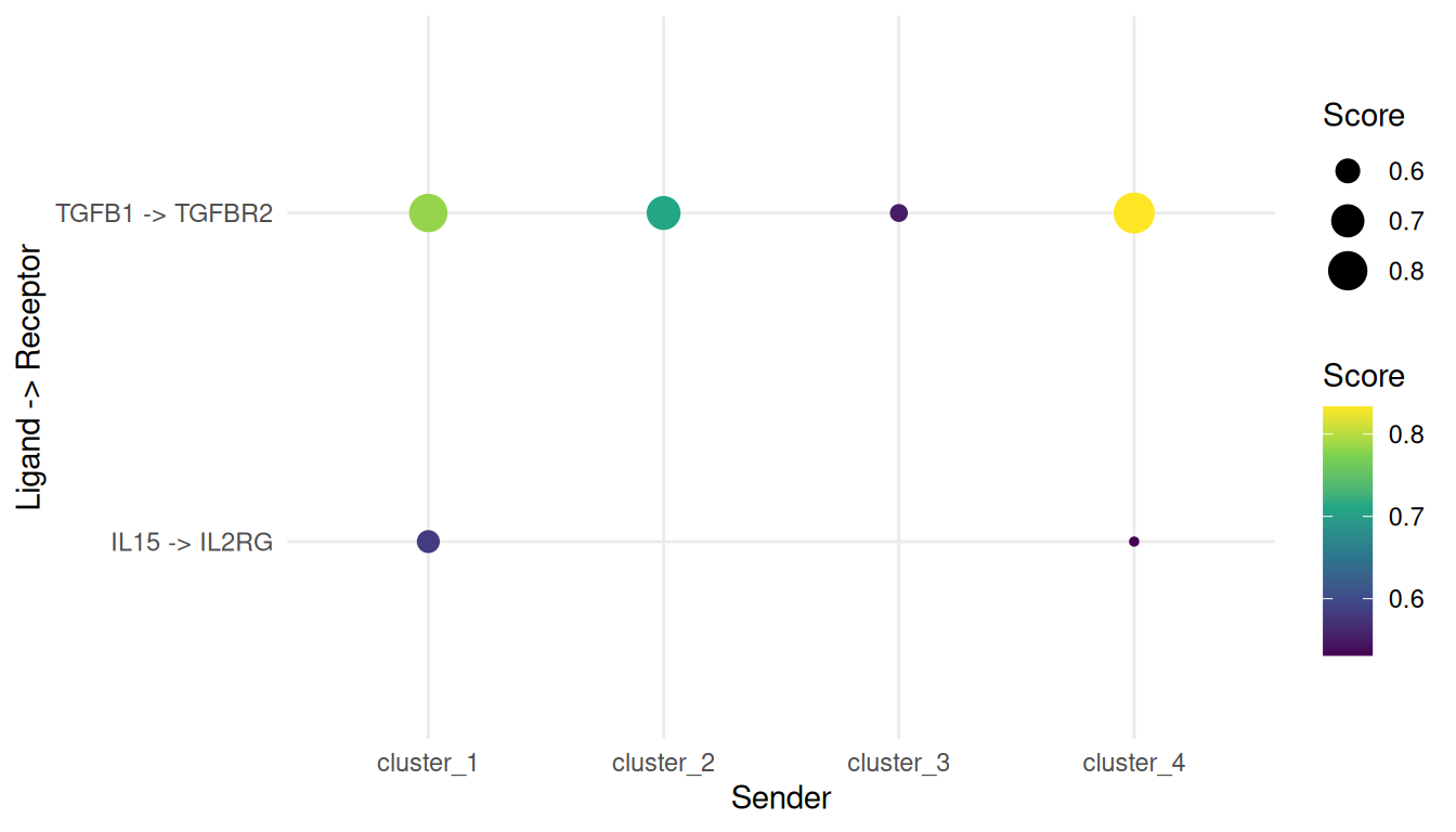
A quick dotplot of the top prioritised interactions.
top_n <- 15L

plot_dt <- head(result, top_n)[, `:=`(
  interaction = paste(ligand_symbol, "->", receptor_symbol)
)]

ggplot(
  plot_dt,
  aes(
    x = sender,
    y = interaction,
    size = prioritisation_score,
    colour = prioritisation_score
  )
) +
  geom_point() +
  scale_colour_viridis_c() +
  theme_minimal() +
  labs(
    x = "Sender",
    y = "Ligand -> Receptor",
    size = "Score",
    colour = "Score"
  )
Notes on DE methods
find_all_markers_sc() runs a Wilcoxon test, which is convenient but inflates p-values in single cell data: each cell is treated as an independent observation. For inference that matters, go pseudo-bulk with DESeq2 or edgeR:
- Aggregate counts per (sample, cluster) into pseudo-bulk.
- Run a standard bulk DE pipeline.
- Feed the result into
cellphonedb_sc(method = "degs")as acluster_id,genetable, or intoprioritise_interactions()after renaming the columns tocluster_id,gene,lfc,pval.
Neither function cares which method produced the DE table.
Clean up
unlink(tempdir_pbmc, recursive = TRUE, force = TRUE)