library(bixverse)
library(bixverse.plots)
library(data.table)
#>
#> Attaching package: 'data.table'
#> The following object is masked from 'package:base':
#>
#>     %notin%
library(ggplot2)
library(magrittr)
Reference mapping with Symphony
2026-09-24
Intro
Once you have a well-annotated reference data set, you usually do not want to re-do the whole pipeline… QC, HVG selection, PCA, batch correction, clustering, manual annotation… And that every time a new sample lands on your desk. Symphony (Kang, et al., 2021) addresses this by compressing the reference into a small set of cached terms that can be used to map new query cells into the same coordinate system in a single shot, with no need to retain the original reference cells at query time.
This vignette walks through the full workflow:
- Build a reference from two PBMC data sets (pbmc3k + pbmc4k), correcting the batch effect with Harmony v2 and annotating cell types with scType.
- Compress the reference into a
SymphonyReferenceand snapshot the cell type labels into it. - Load a third PBMC data set (pbmc8k) as the query, project it through the reference, and transfer labels via kNN majority vote.
If you have not read the batch correction vignette and the introductory vignette, please do so first; this vignette assumes familiarity with both.
Building the reference
Loading the reference batches
We use the same pbmc3k + pbmc4k pair as in the batch correction vignette. Two batches with the same broad cell type composition and a clear technical difference between them is exactly the situation Symphony is designed for: the reference learns the batch correction once, and that correction can then be applied to future queries without rerunning Harmony.
Code
dir_data <- download_pbmc_batches()

tempdir_ref <- file.path(tempdir(), "symphony_ref")
dir.create(tempdir_ref, showWarnings = FALSE, recursive = TRUE)

h5ad_files <- list.files(dir_data)
h5ad_files <- h5ad_files[grepl(".h5ad", h5ad_files)]
h5ad_paths <- file.path(dir_data, h5ad_files)
names(h5ad_paths) <- c("pbmc3k", "pbmc4k")

h5_tasks <- prescan_h5ad_files(h5_paths = h5ad_paths)

sc_ref <- SingleCells(dir_data = tempdir_ref)

sc_ref <- load_multi_h5ad(
  object = sc_ref,
  prescan_result = h5_tasks,
  .verbose = TRUE
)
#>  Using light streaming for the CSR to CSC conversion.
#> Loading observation data from h5ad files into DuckDB.
#> Loading variable data into DuckDB.
Quality control
Standard QC: mitochondrial gene proportions, library complexity, MAD-based outlier detection.
Code
var_ref <- get_sc_var(sc_ref)

# let's get the gene symbols from one of the h5ad files - in multi file import
# additional columns are dropped from the vars
h5_metadata <- read_h5ad_metadata(h5ad_paths[[1]])

var_ref <- merge(
  var_ref,
  h5_metadata$var[, c("ENSEMBL_ID", "Symbol_TENx")],
  by.x = "gene_id",
  by.y = "ENSEMBL_ID"
)

setnames(var_ref, old = "Symbol_TENx", new = "gene_symbol", skip_absent = TRUE)

gs_of_interest <- list(
  MT = var_ref[grepl("^MT-", gene_symbol), gene_id],
  Ribo = var_ref[grepl("^RPS|^RPL", gene_symbol), gene_id]
)

sc_ref <- gene_set_proportions_sc(
  sc_ref,
  gs_of_interest,
  streaming = FALSE,
  .verbose = TRUE
)

qc_df <- sc_ref[[c("cell_id", "lib_size", "nnz", "MT", "exp_id")]]

metrics <- list(
  log10_lib_size = log10(qc_df$lib_size),
  log10_nnz = log10(qc_df$nnz),
  MT = qc_df$MT
)
directions <- c(
  log10_lib_size = "twosided",
  log10_nnz = "twosided",
  MT = "above"
)

qc <- run_cell_qc(
  metrics = metrics,
  cells_to_keep = get_cells_to_keep(sc_ref),
  directions = directions,
  threshold = 3
)

sc_ref[["outlier"]] <- qc$combined
cells_to_keep <- qc_df[!qc$combined, cell_id]
sc_ref <- set_cells_to_keep(sc_ref, cells_to_keep)
HVGs, PCA, Harmony v2
This block is essentially the Harmony v2 path of the batch correction vignette: pick HVGs, run PCA, run Harmony v2, build a neighbour graph on the corrected embedding.
sc_ref <- find_hvg_sc(
  object = sc_ref,
  hvg_no = 2000L,
  .verbose = TRUE
)

sc_ref <- calculate_pca_sc(
  object = sc_ref,
  no_pcs = 30L
)
#> Using dense SVD solving on scaled data on 2000 HVG.

sc_ref <- harmony_v2_sc(
  object = sc_ref,
  batch_column = "exp_id",
  harmony_params = params_sc_harmony_v2()
)
#>  Auto-determined number of Harmony clusters: 100

sc_ref <- find_neighbours_sc(
  object = sc_ref,
  embd_to_use = "harmony_v2",
  neighbours_params = params_sc_neighbours()
)
#>
#> Generating sNN graph (full: TRUE).
#> Transforming sNN data to igraph.
We use Harmony v2 throughout. Version 1 is still available via harmony_sc() and params_sc_harmony(), but v2 is preferable in most settings (see the batch correction vignette for the reasoning).
Clustering and scType annotation
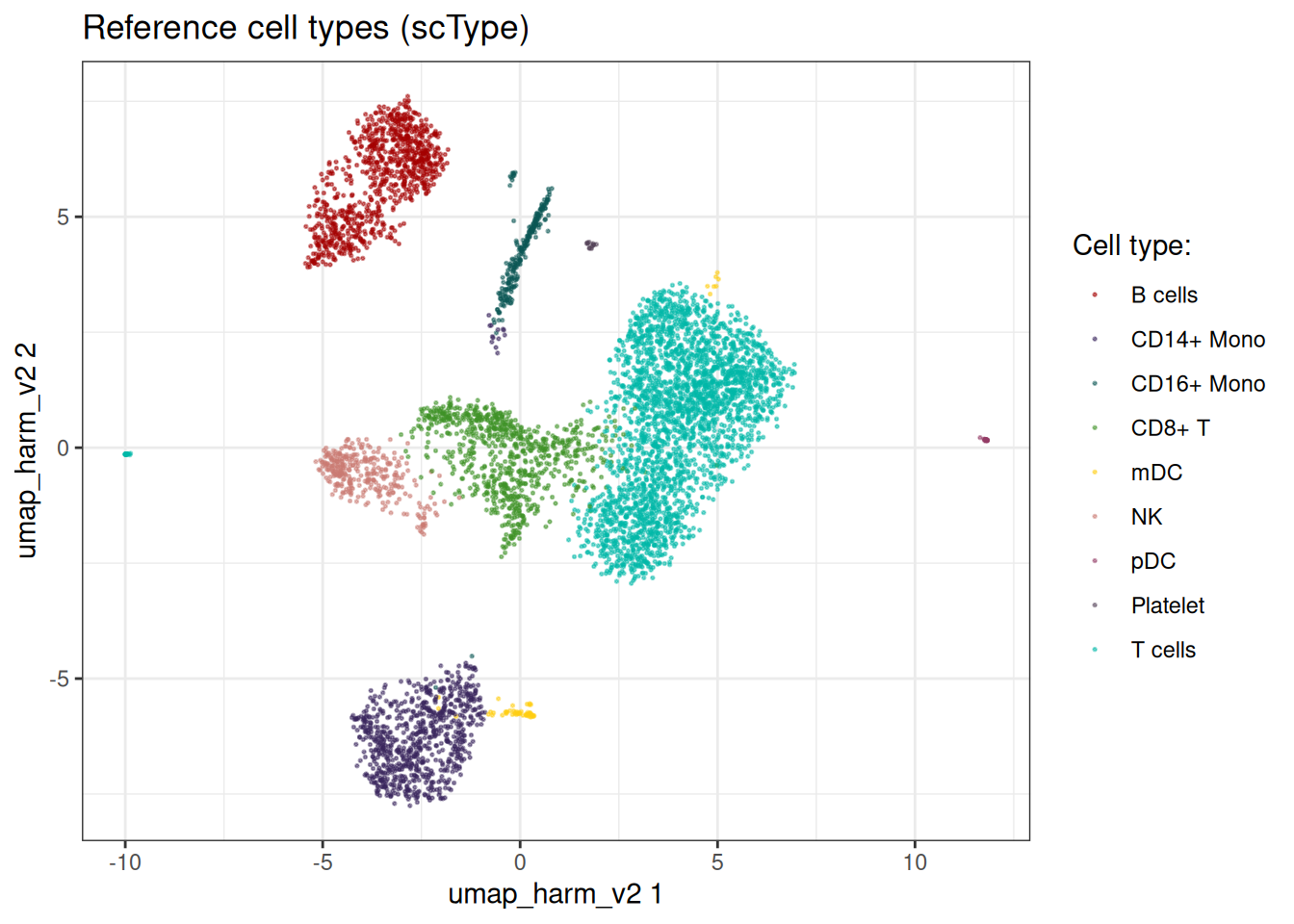
Cluster on the Harmony-corrected graph, then annotate the clusters with scType using a PBMC marker set. This mirrors the annotation block in the PBMC vignette.
sc_ref <- find_clusters_sc(sc_ref, res = 0.5, name = "leiden_clusters")

sc_ref <- umap_sc(
  sc_ref,
  slot_name = "umap_harm_v2",
  use_knn = TRUE
)
#> Running UMAP.
#> Using n_epochs = 500 (dataset <10k samples or adam_parallel optimiser)
#> Using provided kNN graph.
Marker set:
cell_markers <- c(
  CD3D = "T cells",
  CD3E = "T cells",
  CD3G = "T cells",
  IL7R = "CD4+ T",
  CD4 = "CD4+ T",
  CD8A = "CD8+ T",
  CD8B = "CD8+ T",
  MS4A1 = "B cells",
  CD79A = "B cells",
  CD19 = "B cells",
  CD14 = "CD14+ Mono",
  LYZ = "CD14+ Mono",
  S100A8 = "CD14+ Mono",
  FCGR3A = "CD16+ Mono",
  CDKN1C = "CD16+ Mono",
  GNLY = "NK",
  NKG7 = "NK",
  NCAM1 = "NK",
  FCER1A = "mDC",
  CD1C = "mDC",
  LILRA4 = "pDC",
  CLEC4C = "pDC",
  PPBP = "Platelet",
  PF4 = "Platelet"
)
scType scoring and per-cluster assignment:
cell_markers_dt <- stack(cell_markers) %>%
  as.data.table() %>%
  setnames(., c("values", "ind"), c("cell_type", "gene_symbol")) %>%
  .[, gene_symbol := as.character(gene_symbol)] %>%
  .[, gene_id := var_ref$gene_id[match(gene_symbol, var_ref$gene_symbol)]] %>%
  .[!is.na(gene_id), ]

marker_list <- prepare_cell_markers(sc_ref, cell_markers_dt)

sctype_scores <- calc_sc_type_scores(
  object = sc_ref,
  cell_marker_list = marker_list
)

cell_type_anno <- score_clusters(
  sctype_scores,
  sc_ref[[]][["leiden_clusters"]]
)

obs <- get_sc_obs(sc_ref, filtered = TRUE)[, .(
  cell_idx,
  leiden_clusters
)] %>%
  .[,
    sc_type := cell_type_anno$cell_type[match(
      leiden_clusters,
      cell_type_anno$cluster_id
    )]
  ]

sc_ref[["sc_type"]] <- obs$sc_type
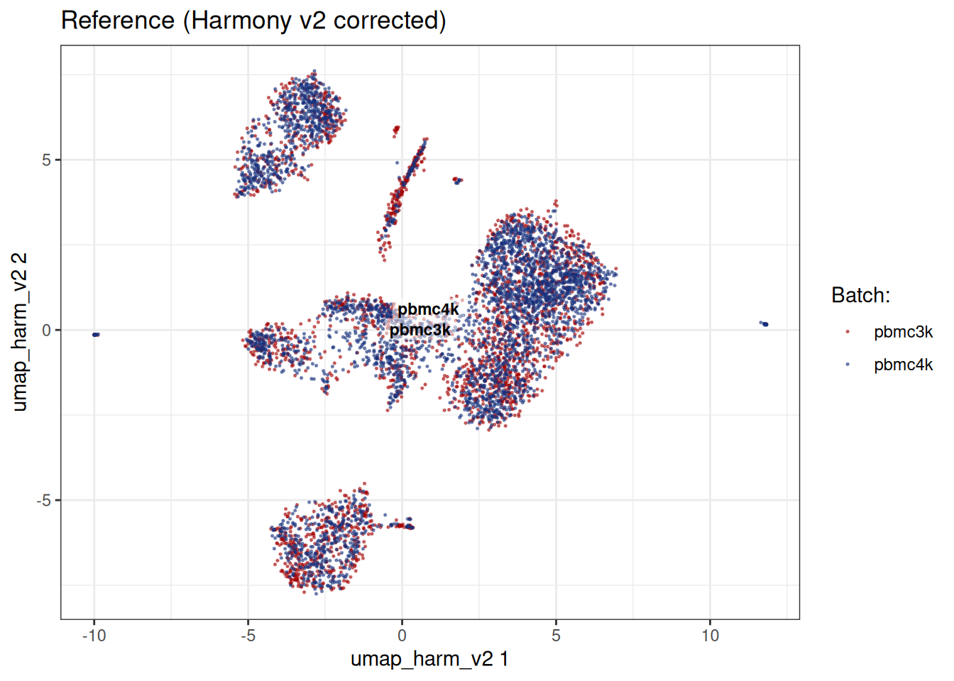
Quick sanity check on the reference: batches mixed, cell types separated.
embedding_plot_sc(
  sc_ref,
  embedding = "umap_harm_v2",
  colour_by = "exp_id",
  label_by = "exp_id",
  discrete = TRUE
) +
  labs(
    title = "Reference (Harmony v2 corrected)",
    colour = "Batch:"
  )
embedding_plot_sc(
  sc_ref,
  embedding = "umap_harm_v2",
  colour_by = "sc_type",
  discrete = TRUE
) +
  labs(
    title = "Reference cell types (scType)",
    colour = "Cell type:"
  )
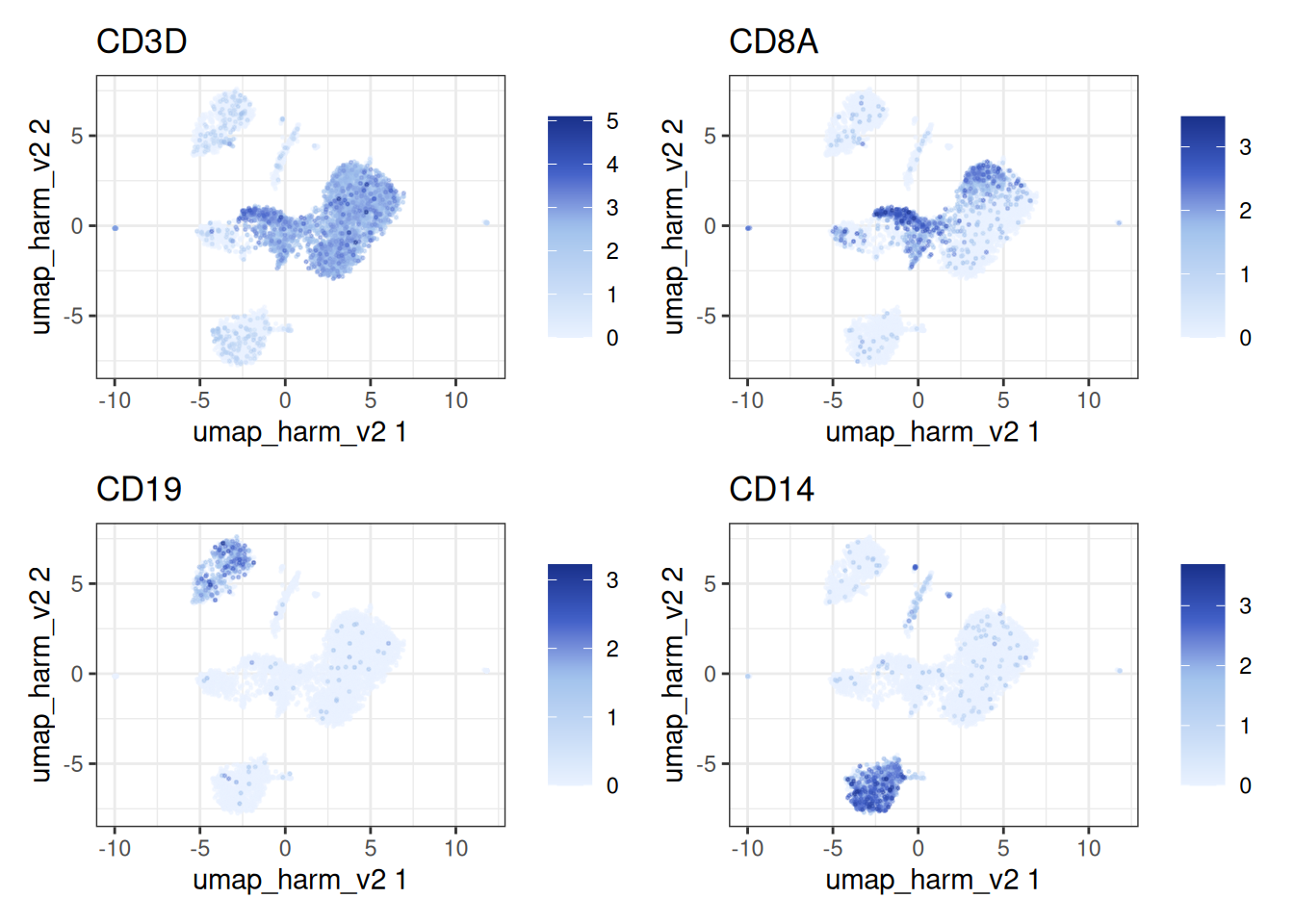
Let’s see how sensible the cell type labels are with some canonical markers
feature_plot_sc(
  object = sc_ref,
  features = c(
    "ENSG00000167286",
    "ENSG00000153563",
    "ENSG00000177455",
    "ENSG00000170458"
  ),
  feature_labels = c(
    "ENSG00000167286" = "CD3D",
    "ENSG00000153563" = "CD8A",
    "ENSG00000177455" = "CD19",
    "ENSG00000170458" = "CD14"
  ),
  embedding = "umap_harm_v2"
)
Compressing into a SymphonyReference
We now have everything we need: HVG selection, batch annotation, cell type labels in the obs table. build_symphony_ref() re-runs PCA and Harmony internally using the supplied HVGs, then caches the loadings, centroids and compression terms (Nr, C) needed for query mapping. Pass label_columns to snapshot one or more obs columns – here the scType annotation – into the reference for downstream label transfer.
A note on the apparent duplication: yes, indeed, PCA + Harmony are run again inside build_symphony_ref(), even though we just ran them on the same HVGs in the preprocessing block above. This is deliberate. The standard pipeline keeps its embeddings on the SingleCells object and streams from disk; the Symphony reference keeps a self-contained, in-memory copy of everything it needs to project queries without the reference cells. Sharing state across those two representations would tie them together in unhelpful ways. The cost is one extra PCA + Harmony run at build time while avoiding coupling between the methods.
hvg_indices <- get_hvg(sc_ref) + 1L

symphony_ref <- build_symphony_ref(
  object = sc_ref,
  batch_column = "exp_id",
  hvg = hvg_indices,
  harmony_params = params_sc_harmony_v2(),
  pca_params = params_sc_pca(),
  no_pcs = 30L,
  label_columns = "sc_type",
  .verbose = TRUE
)
#>  Auto-determined number of Harmony clusters: 100

symphony_ref
#> Symphony reference
#>   Harmony backend: v2
#>   No HVGs: 2000
#>   No PCs: 30
#>   No clusters: 100
#>   Batch variables: exp_id
#>   Slim: FALSE
#>   Labels: sc_type
The print method tells you the Harmony backend, the size of the loadings and centroid matrices, the batch variables and the stored label columns.
Mapping a query
Loading the query
We use pbmc8k as the query. Same tissue, same broad biology, but a different 10x run – exactly the kind of “another sample arrives” scenario Symphony is built for.
Code
pbmc8k_path <- download_pbmc8k()

tempdir_query <- file.path(tempdir(), "symphony_query")
dir.create(tempdir_query, showWarnings = FALSE, recursive = TRUE)

mtx_io_params <- get_cell_ranger_params(pbmc8k_path)

sc_query <- SingleCells(dir_data = tempdir_query)

sc_query <- load_mtx(
  object = sc_query,
  sc_mtx_io_param = mtx_io_params,
  mtx_streaming = FALSE,
  .verbose = TRUE
)
#>  Using light streaming for the CSR to CSC conversion.
#> Loading observations data from flat file into the DuckDB.
#> Loading variable data from flat file into the DuckDB.
Quality control on the query
Same QC as the reference. We are not trying to match library sizes or anything fancy across data sets – just remove clearly bad cells.
Code
var_q <- get_sc_var(sc_query)

gs_q <- list(
  MT = var_q[grepl("^MT-", column1), gene_id],
  Ribo = var_q[grepl("^RPS|^RPL", column1), gene_id]
)

sc_query <- gene_set_proportions_sc(
  sc_query,
  gs_q,
  streaming = FALSE,
  .verbose = TRUE
)

qc_df_q <- sc_query[[c("cell_id", "lib_size", "nnz", "MT")]]

metrics_q <- list(
  log10_lib_size = log10(qc_df_q$lib_size),
  log10_nnz = log10(qc_df_q$nnz),
  MT = qc_df_q$MT
)

qc_q <- run_cell_qc(
  metrics = metrics_q,
  cells_to_keep = get_cells_to_keep(sc_query),
  directions = c(
    log10_lib_size = "twosided",
    log10_nnz = "twosided",
    MT = "above"
  ),
  threshold = 3
)

sc_query[["outlier"]] <- qc_q$combined
sc_query <- set_cells_to_keep(
  sc_query,
  qc_df_q[!qc_q$combined, cell_id]
)
Projecting the query
map_symphony_query() does the actual projection: query cells are standardised against the reference’s per-HVG means and SDs, projected through the reference PCA loadings, and assigned soft cluster weights against the reference centroids. Those weights then drive the cached MoE batch correction, putting query cells into the same z_corr coordinate system as the reference.
Genes are matched by name. Missing HVGs are treated as zero columns; the function reports how many were missing.
Even though pbmc8k is a single batch, we still pass batch_column = "exp_id" so Symphony applies the cached correction relative to the reference batches. Setting batch_column = NULL skips correction entirely (the resulting symphony embedding then equals symphony_pca).
sc_query <- map_symphony_query(
  reference = symphony_ref,
  query = sc_query,
  batch_column = NULL,
  params = params_symphony_map(),
  .verbose = TRUE
)
#>  17 / 2000 reference HVGs not found in query; treated as zero columns.
The query now carries three embeddings: "symphony" (z_corr, the corrected embedding), "symphony_pca" (z_pca, pre-correction), and "symphony_r" (soft cluster assignments, one column per reference centroid).
A neighbour graph and UMAP on the corrected embedding give us something to plot against:
sc_query <- find_neighbours_sc(
  object = sc_query,
  embd_to_use = "symphony",
  neighbours_params = params_sc_neighbours()
)
#>
#> Generating sNN graph (full: TRUE).
#> Transforming sNN data to igraph.

sc_query <- umap_sc(
  sc_query,
  embd_to_use = "symphony",
  slot_name = "umap_symphony",
  use_knn = TRUE
)
#> Running UMAP.
#> Using n_epochs = 500 (dataset <10k samples or adam_parallel optimiser)
#> Using provided kNN graph.
Transferring labels
transfer_labels_symphony() does a kNN majority vote on the reference’s z_corr (the searchable index) using the query’s "symphony" embedding. It reads labels directly from the reference’s stored labels slot – the one we populated via label_columns = "sc_type" at build time.
Distances on z_corr are typically Euclidean; the default params_sc_knn() matches.
predicted <- transfer_labels_symphony(
  reference = symphony_ref,
  query = sc_query,
  label_column = "sc_type",
  knn_params = params_sc_knn(),
  .verbose = TRUE
)

head(predicted)
#>    predicted_sc_type confidence_sc_type
#>               <char>              <num>
#> 1:           B cells                  1
#> 2:           T cells                  1
#> 3:           T cells                  1
#> 4:        CD14+ Mono                  1
#> 5:        CD14+ Mono                  1
#> 6:            CD8+ T                  1
The result is a data.table in get_cells_to_keep(query) order with a predicted label and a confidence score (fraction of neighbours agreeing on the winning class). We can attach both directly to the query obs.
Visualising the result
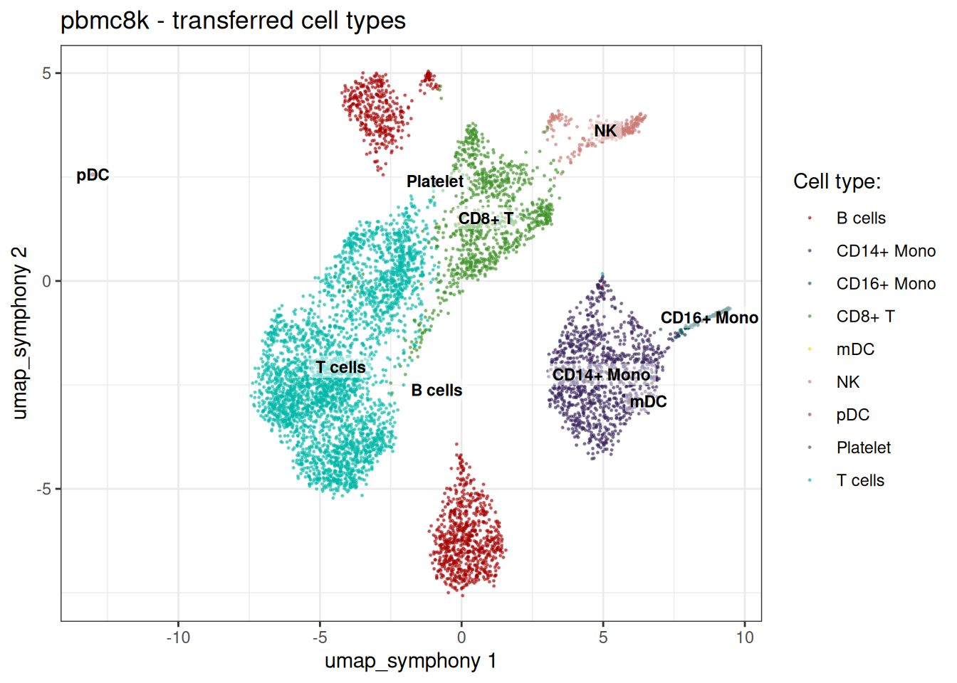
Query UMAP coloured by transferred cell type:
embedding_plot_sc(
  sc_query,
  embedding = "umap_symphony",
  colour_by = "predicted_sc_type",
  label_by = "predicted_sc_type",
  discrete = TRUE
) +
  labs(
    title = "pbmc8k - transferred cell types",
    colour = "Cell type:"
  )
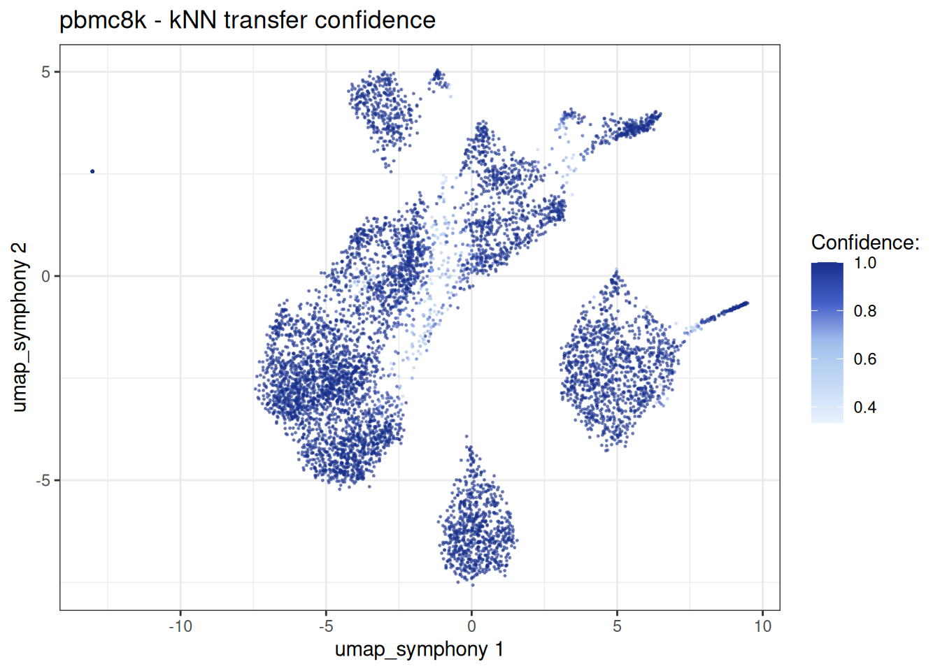
Same UMAP, but coloured by transfer confidence. Cells in the “interior” of their cell type usually have confidence 1; cells sitting on cluster boundaries or in cell types poorly represented in the reference are the ones to scrutinise.
embedding_plot_sc(
  sc_query,
  embedding = "umap_symphony",
  colour_by = "sc_type_confidence",
  discrete = FALSE
) +
  labs(
    title = "pbmc8k - kNN transfer confidence",
    colour = "Confidence:"
  )
And a per-cell-type confidence distribution – useful for spotting cell types where the reference and query disagree systematically:
conf_dt <- sc_query[[c("predicted_sc_type", "sc_type_confidence")]]

ggplot(conf_dt, aes(x = predicted_sc_type, y = sc_type_confidence)) +
  geom_violin(scale = "width", fill = "grey80") +
  geom_jitter(width = 0.15, alpha = 0.2, size = 0.4) +
  labs(
    x = NULL,
    y = "Transfer confidence",
    title = "Per-cell-type kNN agreement on pbmc8k"
  ) +
  theme_minimal() +
  theme(axis.text.x = element_text(angle = 30, hjust = 1)) +
  ylim(0, 1.025)
#> Warning: Groups with fewer than two datapoints have been dropped.
#> ℹ Set `drop = FALSE` to consider such groups for position adjustment purposes.
#> Warning: Removed 207 rows containing missing values or values outside the scale range
#> (`geom_point()`).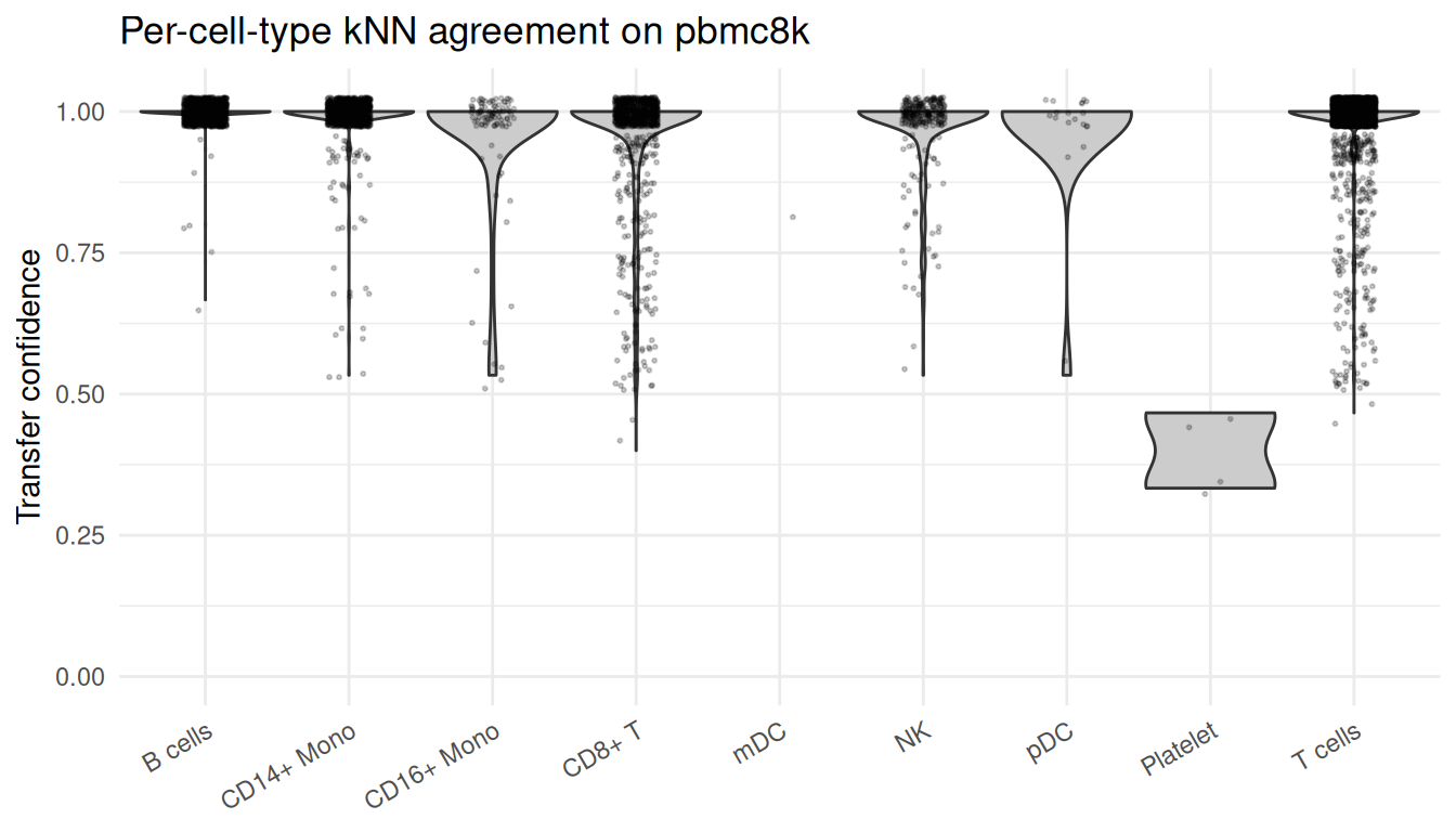
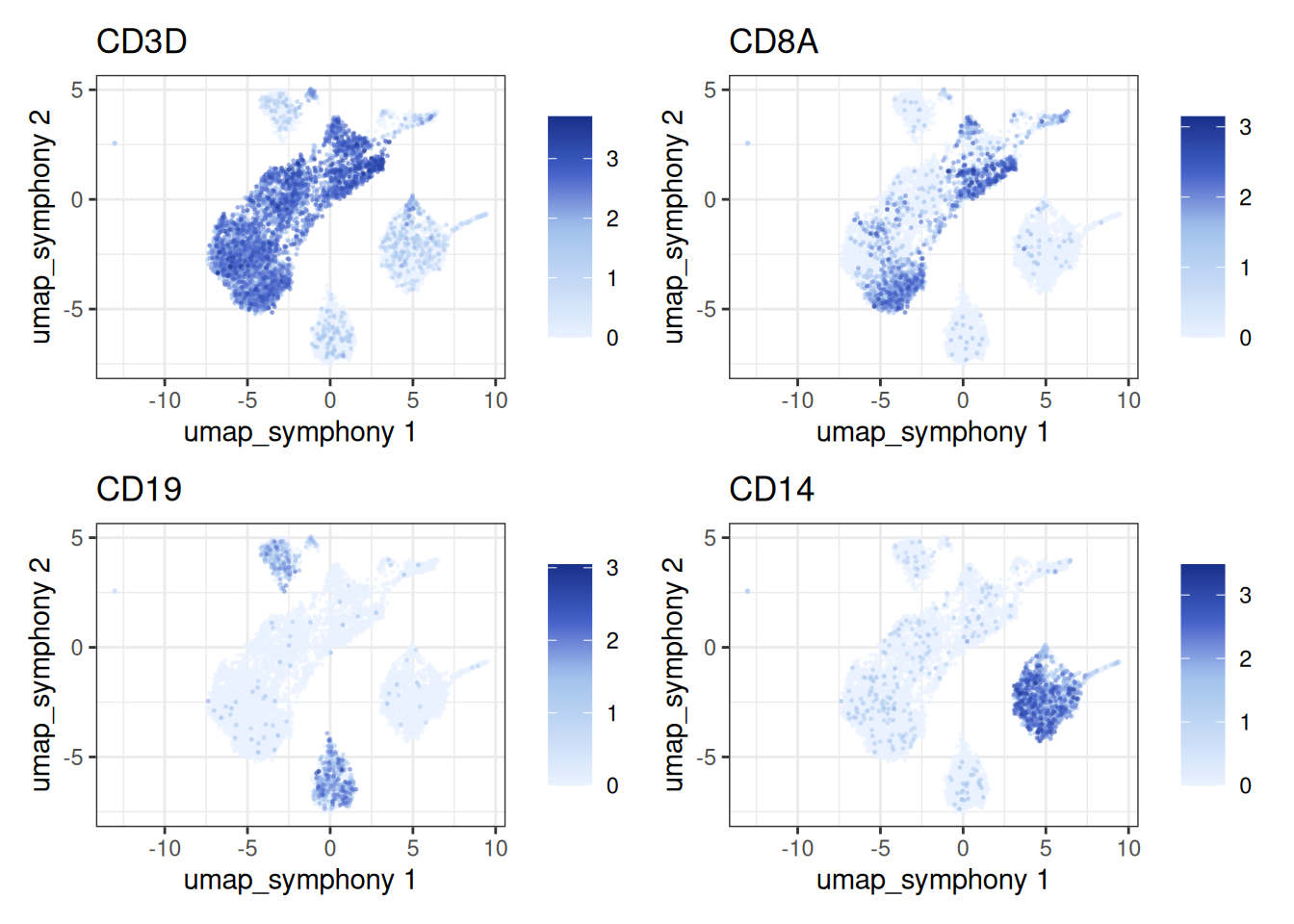
Let’s also sanity check the label propagation with some canonical markers:
feature_plot_sc(
  object = sc_query,
  features = c(
    "ENSG00000167286",
    "ENSG00000153563",
    "ENSG00000177455",
    "ENSG00000170458"
  ),
  feature_labels = c(
    "ENSG00000167286" = "CD3D",
    "ENSG00000153563" = "CD8A",
    "ENSG00000177455" = "CD19",
    "ENSG00000170458" = "CD14"
  ),
  embedding = "umap_symphony"
)
Slim references and post-hoc labels
The reference above stores z_corr, z_orig, the soft cluster assignments r and the labels. For large references that get checked into shared storage, z_orig and r are usually dead weight; passing slim = TRUE at build time drops them. z_corr is always retained – it is what kNN label transfer searches against.
If you want to add or update labels after the reference is already built (say, you re-ran scType with a different marker set), use add_symphony_labels(). It reads obs columns from a SingleCells object in cells_to_keep order and snapshots them into the reference. The cells_to_keep state must match the reference – the function enforces this with a hard error if the row count drifts.
slim_ref <- build_symphony_ref(
  object = sc_ref,
  batch_column = "exp_id",
  hvg = hvg_indices,
  harmony_params = params_sc_harmony_v2(),
  pca_params = params_sc_pca(),
  no_pcs = 30L,
  slim = TRUE
)

slim_ref <- add_symphony_labels(
  reference = slim_ref,
  sc_object = sc_ref,
  columns = "sc_type"
)
Multiple label columns can be attached at once (columns = c(...)), existing columns are protected unless you pass overwrite = TRUE, and get_symphony_labels(reference) returns the stored data.table (or NULL if none).