
NicheNet ligand-receptor analysis with bixverse
2026-09-24
Intro
This vignette walks through a NicheNet-style ligand-receptor analysis on the PBMC3k data set using bixverse. It assumes familiarity with the SingleCells class and the basic processing pipeline; if you have not read the PBMC processing vignette, please do so first.
NicheNet ranks upstream ligands by how well their predicted target gene sets align with a gene set of interest in a receiver cell type. The pipeline here is:
- Build a ligand-target regulatory potential matrix from a signalling network (PPI) and a gene regulatory network (GRN).
- Define a gene set of interest in the receiver (here, T-cell marker genes).
- Score each ligand by how well its targets overlap with that gene set (AUROC, AUPR, correlations).
- Combine ligand activity with sender/receiver expression and DE into a single prioritisation score.
Loading and processing PBMC3k
We reuse the standard processing pipeline. See the PBMC processing vignette for commentary on each step.
pbmc3k_path <- download_pbmc3k()
tempdir_pbmc <- tempdir()

sc_object <- SingleCells(dir_data = tempdir_pbmc)
mtx_io_params <- get_cell_ranger_params(pbmc3k_path)

sc_object <- load_mtx(
  object = sc_object,
  sc_mtx_io_param = mtx_io_params,
  mtx_streaming = FALSE,
  .verbose = FALSE
)

setnames_sc(sc_object, table = "var", old = "column1", new = "gene_symbol")
var <- get_sc_var(sc_object)
symbol_to_ensembl <- setNames(var$gene_id, var$gene_symbol)
ensembl_to_symbol <- setNames(var$gene_symbol, var$gene_id)

# QC and processing
gs_of_interest <- list(
  MT = var[grepl("^MT-", gene_symbol), gene_id],
  Ribo = var[grepl("^RPS|^RPL", gene_symbol), gene_id]
)
sc_object <- gene_set_proportions_sc(
  sc_object,
  gs_of_interest,
  .verbose = FALSE
)

# minimal cell filtering
cells_to_keep <- sc_object[[]][MT < 0.2, cell_id]
sc_object <- set_cells_to_keep(sc_object, cells_to_keep)

sc_object <- find_hvg_sc(sc_object, hvg_no = 2000L, .verbose = FALSE)
sc_object <- calculate_pca_sc(sc_object, no_pcs = 30L, .verbose = FALSE)
sc_object <- find_neighbours_sc(sc_object, .verbose = FALSE)
sc_object <- find_clusters_sc(sc_object, res = 0.5)
For demonstration purposes we use the Leiden cluster IDs directly as cell types. In a real analysis you would annotate clusters via marker genes (e.g. with find_all_markers_sc and a canonical marker panel) before running prioritisation; senders and receivers are biological concepts.
sc_object[["celltype"]] <- paste0(
  "cluster_",
  unlist(sc_object[["leiden_clustering"]])
)

celltype_counts <- sc_object[[]][!is.na(celltype), .N, by = celltype][order(-N)]

celltype_counts
#>     celltype     N
#>       <char> <int>
#> 1: cluster_0  1207
#> 2: cluster_1   491
#> 3: cluster_2   444
#> 4: cluster_3   348
#> 5: cluster_4   161
#> 6: cluster_5    32
#> 7: cluster_6    15
Building the NicheNet networks
A production analysis would load the curated NicheNet networks (signalling + GRN) from Zenodo. For a self-contained vignette we construct a small network covering a handful of canonical immune-signalling pathways. The shape of the inputs is what matters here… Also, this allows you to feed in your own networks if desired.
# Ligand-receptor pairs (canonical immune signalling)
lr_network <- data.table(
  # ligands
  from = c("CCL5", "CXCL10", "IL15", "TNF", "TGFB1", "IL10", "ICAM1"),
  # receptors
  to = c(
    "CCR5",
    "CXCR3",
    "IL2RG",
    "TNFRSF1A",
    "TGFBR2",
    "IL10RA",
    "ITGAL"
  ),
  weight = 1
)

# Signalling (PPI) layer: ligand -> receptor -> intracellular signalling -> TFs
ppi_network <- data.table(
  from = c(
    "CCL5",
    "CXCL10",
    "IL15",
    "TNF",
    "TGFB1",
    "IL10",
    "ICAM1",
    "CCR5",
    "CXCR3",
    "IL2RG",
    "TNFRSF1A",
    "TGFBR2",
    "IL10RA",
    "ITGAL",
    "JAK1",
    "JAK2",
    "JAK3",
    "STAT1",
    "STAT3",
    "STAT5A",
    "NFKB1",
    "SMAD2"
  ),
  to = c(
    "CCR5",
    "CXCR3",
    "IL2RG",
    "TNFRSF1A",
    "TGFBR2",
    "IL10RA",
    "ITGAL",
    "JAK1",
    "JAK1",
    "JAK3",
    "NFKB1",
    "SMAD2",
    "JAK1",
    "NFKB1",
    "STAT1",
    "STAT3",
    "STAT5A",
    "STAT3",
    "STAT1",
    "STAT3",
    "STAT3",
    "STAT3"
  ),
  weight = 1
)

# GRN layer: TF -> targets
grn_network <- data.table(
  from = c(
    rep("STAT1", 6),
    rep("STAT3", 6),
    rep("STAT5A", 4),
    rep("NFKB1", 6),
    rep("SMAD2", 4)
  ),
  to = c(
    "IRF1",
    "MX1",
    "ISG15",
    "OAS1",
    "GBP1",
    "CXCL10",
    "SOCS3",
    "IL6",
    "BCL2",
    "VEGFA",
    "MYC",
    "FOS",
    "CCND1",
    "BCL2L1",
    "IL2RA",
    "FOXP3",
    "TNF",
    "IL1B",
    "IL6",
    "NFKBIA",
    "CCL5",
    "ICAM1",
    "SERPINE1",
    "CDKN1A",
    "JUNB",
    "ID1"
  ),
  weight = 1
)
Map gene symbols to the Ensembl IDs used internally by sc_object, dropping any genes not present in the data set.
symbol_to_id <- function(syms) {
  ids <- symbol_to_ensembl[syms]
  ids[!is.na(ids)]
}

# Restrict the networks to genes present in PBMC3k
keep_ppi <- ppi_network$from %in%
  names(symbol_to_ensembl) &
  ppi_network$to %in% names(symbol_to_ensembl)
keep_grn <- grn_network$from %in%
  names(symbol_to_ensembl) &
  grn_network$to %in% names(symbol_to_ensembl)
keep_lr <- lr_network$from %in%
  names(symbol_to_ensembl) &
  lr_network$to %in% names(symbol_to_ensembl)

ppi_network <- ppi_network[keep_ppi]
grn_network <- grn_network[keep_grn]
lr_network <- lr_network[keep_lr]
Ligand-target regulatory potential
Construct the ligand-target influence matrix. Each row is one ligand and each column is a gene from the union of both networks; entries are NicheNet-style regulatory potential scores.
ligand_seeds <- setNames(
  lapply(lr_network$from, identity),
  lr_network$from
)

ligand_influence <- generate_ligand_target_influence(
  ligand_seeds = ligand_seeds,
  ppi_network = rbind(lr_network, ppi_network),
  grn_network = grn_network,
  # because of the tiny network, the original ltf_cutoff of 0.99 would be way
  # too aggressive
  params = params_ligand_target(ltf_cutoff = 0)
)

ligand_influence
#> LigandTargetInfluence
#>   No ligand seeds:    6
#>   No genes:           40
#>   Damping factor:     0.500
#>   Max iter:           1000
#>   Secondary targets:  FALSE
This returns a LigandTargetInfluence class. If you want to access the actual scores, you can use:
get_influence(ligand_influence)
#>         CCL5     CXCL10 IL15   TNF TGFB1 ICAM1 CCR5 CXCR3 IL2RG TNFRSF1A TGFBR2
#> CCL5   0.000 0.08349609    0 0.000     0 0.000    0     0     0        0      0
#> CXCL10 0.000 0.08349609    0 0.000     0 0.000    0     0     0        0      0
#> IL15   0.000 0.02099609    0 0.000     0 0.000    0     0     0        0      0
#> TNF    0.125 0.04150391    0 0.125     0 0.125    0     0     0        0      0
#> TGFB1  0.000 0.04150391    0 0.000     0 0.000    0     0     0        0      0
#> ICAM1  0.125 0.04150391    0 0.125     0 0.125    0     0     0        0      0
#>        IL10RA ITGAL JAK1 JAK2 JAK3 STAT1 STAT3 STAT5A NFKB1 SMAD2       IRF1
#> CCL5        0     0    0    0    0     0     0      0     0     0 0.08349609
#> CXCL10      0     0    0    0    0     0     0      0     0     0 0.08349609
#> IL15        0     0    0    0    0     0     0      0     0     0 0.02099609
#> TNF         0     0    0    0    0     0     0      0     0     0 0.04150391
#> TGFB1       0     0    0    0    0     0     0      0     0     0 0.04150391
#> ICAM1       0     0    0    0    0     0     0      0     0     0 0.04150391
#>               MX1      ISG15       OAS1       GBP1      SOCS3        IL6
#> CCL5   0.08349609 0.08349609 0.08349609 0.08349609 0.04150391 0.04150391
#> CXCL10 0.08349609 0.08349609 0.08349609 0.08349609 0.04150391 0.04150391
#> IL15   0.02099609 0.02099609 0.02099609 0.02099609 0.04150391 0.04150391
#> TNF    0.04150391 0.04150391 0.04150391 0.04150391 0.08349609 0.20849609
#> TGFB1  0.04150391 0.04150391 0.04150391 0.04150391 0.08349609 0.08349609
#> ICAM1  0.04150391 0.04150391 0.04150391 0.04150391 0.08349609 0.20849609
#>              BCL2      VEGFA        MYC        FOS BCL2L1  IL2RA  FOXP3  IL1B
#> CCL5   0.04150391 0.04150391 0.04150391 0.04150391 0.0000 0.0000 0.0000 0.000
#> CXCL10 0.04150391 0.04150391 0.04150391 0.04150391 0.0000 0.0000 0.0000 0.000
#> IL15   0.04150391 0.04150391 0.04150391 0.04150391 0.0625 0.0625 0.0625 0.000
#> TNF    0.08349609 0.08349609 0.08349609 0.08349609 0.0000 0.0000 0.0000 0.125
#> TGFB1  0.08349609 0.08349609 0.08349609 0.08349609 0.0000 0.0000 0.0000 0.000
#> ICAM1  0.08349609 0.08349609 0.08349609 0.08349609 0.0000 0.0000 0.0000 0.125
#>        NFKBIA CDKN1A  JUNB   ID1
#> CCL5    0.000  0.000 0.000 0.000
#> CXCL10  0.000  0.000 0.000 0.000
#> IL15    0.000  0.000 0.000 0.000
#> TNF     0.125  0.000 0.000 0.000
#> TGFB1   0.000  0.125 0.125 0.125
#> ICAM1   0.125  0.000 0.000 0.000
Defining the gene set of interest
In a case/control experiment, the gene set of interest would be the DEGs between conditions in the receiver cell type. PBMC3k is a single condition, so we use cluster-vs-rest marker genes as a stand-in. Pick the largest cluster as receiver and a few others as senders.
receiver_id <- celltype_counts[1, celltype]
senders_oi <- celltype_counts[2:min(5, .N), celltype]

receiver_cells <- sc_object[[]][celltype == receiver_id, cell_id]
other_cells <- sc_object[[]][
  celltype != receiver_id & !is.na(celltype),
  cell_id
]

receiver_de <- find_markers_sc(
  object = sc_object,
  cells_1 = receiver_cells,
  cells_2 = other_cells,
  .verbose = FALSE
)

# upregulated genes with FDR <= 0.05 form the gene set
geneset_oi <- receiver_de[lfc > 0 & fdr <= 0.05, gene_id]
length(geneset_oi)
#> [1] 877
Ligand activity scoring
Score each ligand by how well its target potential vector aligns with geneset_oi. The background is the full set of genes in the influence matrix.
activity <- ligand_activity_scores(
  ligand_influence = ligand_influence,
  # need to transform to gene symbols
  gene_sets = list(receiver_degs = ensembl_to_symbol[geneset_oi])
)

activity[order(-aupr_corrected)]
#>         gene_set ligand     auroc      aupr aupr_corrected      pearson
#>           <char> <char>     <num>     <num>          <num>        <num>
#> 1: receiver_degs  TGFB1 0.6594982 0.3956790    0.170679012  0.300241353
#> 2: receiver_degs   IL15 0.5663082 0.2353395    0.010339506  0.115291205
#> 3: receiver_degs   CCL5 0.5501792 0.2291667    0.004166667 -0.005304068
#> 4: receiver_degs CXCL10 0.5501792 0.2291667    0.004166667 -0.005304068
#> 5: receiver_degs    TNF 0.5125448 0.2086676   -0.016332442 -0.004003802
#> 6: receiver_degs  ICAM1 0.5125448 0.2086676   -0.016332442 -0.004003802
#>      spearman
#>         <num>
#> 1: 0.26664795
#> 2: 0.11085364
#> 3: 0.09001531
#> 4: 0.09001531
#> 5: 0.02025577
#> 6: 0.02025577
Sender and receiver tables
Compute the inputs needed for prioritisation: DE of ligands across senders, DE of receptors in the receiver, and average expression of ligands / receptors per cluster.
celltype_de <- find_all_markers_sc(
  object = sc_object,
  column_of_interest = "celltype",
  .verbose = FALSE
)

# `find_*_markers_sc` returns `gene_id` and `cluster`; rename to match the
# prioritisation function's expected schema.
setnames(
  celltype_de,
  c("gene_id", "grp", "p_values"),
  c("gene", "cluster_id", "pval"),
  skip_absent = TRUE
)
celltype_de <- celltype_de[, .(cluster_id, gene, lfc, pval)]
Compute average expression per cluster for the ligands and receptors of interest. This calls into the streaming engine via compute_expression_info_sc.
genes_of_interest <- union(lr_network$to, lr_network$from)
genes_of_interest_ids <- symbol_to_id(genes_of_interest)

expression_info <- compute_expression_info_sc(
  object = sc_object,
  celltype_colname = "celltype",
  genes = genes_of_interest_ids
)
Prioritisation
Combine all of the above into a single weighted score. PBMC3k has no condition contrast, so we use the "one_condition" scenario, which sets the condition-specificity weights to zero.
# Reduce activity table to one row per ligand (we ran one gene set)
la_input <- activity[, .(ligand, aupr_corrected)]
la_input[, ligand := symbol_to_ensembl[ligand]]

lr_network_ensembl <- data.table(
  ligand = symbol_to_ensembl[lr_network$from],
  receptor = symbol_to_ensembl[lr_network$to]
) %>%
  na.omit()

result <- prioritise_interactions(
  celltype_de = celltype_de,
  expression_info = expression_info,
  ligand_activities = na.omit(la_input),
  lr_network = lr_network_ensembl,
  senders_oi = senders_oi,
  receivers_oi = receiver_id,
  scenario = "one_condition"
)
Add symbol columns for readability.
result[, ligand_symbol := ensembl_to_symbol[ligand]]
result[, receptor_symbol := ensembl_to_symbol[receptor]]

head(
  result[, .(
    sender,
    receiver,
    ligand_symbol,
    receptor_symbol,
    prioritisation_score,
    prioritisation_rank
  )],
  10
)
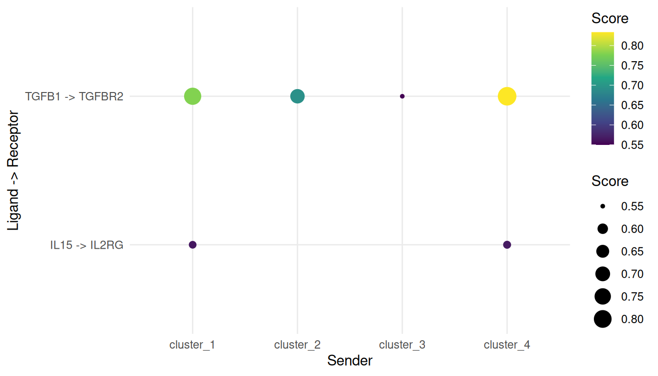
#>       sender  receiver ligand_symbol receptor_symbol prioritisation_score
#>       <char>    <char>        <char>          <char>                <num>
#> 1: cluster_4 cluster_0         TGFB1          TGFBR2            0.8333333
#> 2: cluster_1 cluster_0         TGFB1          TGFBR2            0.7793662
#> 3: cluster_2 cluster_0         TGFB1          TGFBR2            0.6914723
#> 4: cluster_4 cluster_0          IL15           IL2RG            0.5663366
#> 5: cluster_1 cluster_0          IL15           IL2RG            0.5637502
#> 6: cluster_3 cluster_0         TGFB1          TGFBR2            0.5500000
#>    prioritisation_rank
#>                  <int>
#> 1:                   1
#> 2:                   2
#> 3:                   3
#> 4:                   4
#> 5:                   5
#> 6:                   6
Top interactions
A quick dotplot of the top prioritised interactions.
top_n <- 15L

plot_dt <- head(result, top_n)[, `:=`(
  interaction = paste(ligand_symbol, "->", receptor_symbol)
)]

ggplot(
  plot_dt,
  aes(
    x = sender,
    y = interaction,
    size = prioritisation_score,
    colour = prioritisation_score
  )
) +
  geom_point() +
  scale_colour_viridis_c() +
  theme_minimal() +
  labs(
    x = "Sender",
    y = "Ligand -> Receptor",
    size = "Score",
    colour = "Score"
  )
Notes on DE methods
find_markers_sc runs a Wilcoxon-style test, which is convenient but suffers from well-documented p-value inflation in single-cell data (because each cell is treated as an independent observation). For statistical inference that matters, prefer pseudo-bulk + DESeq2 or edgeR:
- Aggregate counts per (sample, cluster) into pseudo-bulk.
- Run a standard bulk DE pipeline.
- Feed the resulting
data.tableintoprioritise_interactionsafter renaming columns tocluster_id,gene,lfc,pval.
The prioritisation function does not care which method produced the DE table.
Clean up
unlink(tempdir_pbmc, recursive = TRUE, force = TRUE)